Difference between revisions of "An initial path towards statistical analysis"
| (38 intermediate revisions by 2 users not shown) | |||
| Line 1: | Line 1: | ||
| − | Learning statistics takes time, as it is mostly experience that allows us to be able to approach the statistical analysis of any given dataset. '''While we cannot take off of you the burden to gather experience yourself, we developed this interactive page for you to find the best statistical method to analyze your given dataset.''' This can be a start for you to dive deeper into statistical analysis, and helps you better design studies.<br/> | + | Learning statistics takes time, as it is mostly experience that allows us to be able to approach the statistical analysis of any given dataset. '''While we cannot take off of you the burden to gather experience yourself, we developed this interactive page for you to find the best statistical method to analyze your given dataset.''' This can be a start for you to dive deeper into statistical analysis, and helps you better [[Designing studies|design studies]].<br/> |
| − | + | <u>This page revolves around statistical analyses of data that has at least two variables.</u> If you only have one variable, e.g. height data of a dozen trees, or your ratings for five types of cake, you might be interested in simpler forms of data analysis and visualisation. Have a look at [[Descriptive statistics]] and [[Introduction to statistical figures]] to see which approaches might work for your data. | |
| − | If you | ||
| + | <u>If you have more than one variable, you have come to the perfect place!</u> <br> | ||
| + | Go through the images step by step, click on the answers that apply to your data, and let the page guide you. <br> | ||
| + | If you need help with data visualisation for any of these approaches, please refer to the entry on [[Introduction to statistical figures]].<br>If you are on mobile and/or just want a list of all entries, please refer to the [[Statistics]] overview page. | ||
| + | ---- | ||
'''Start here with your data! This is your first question.''' | '''Start here with your data! This is your first question.''' | ||
| − | <imagemap> | + | <imagemap>File:Statistics Flowchart - First Step 1.1.png|650px|center| |
| − | poly | + | poly 1120 1020 1580 560 2008 1028 1560 1472 [[An_initial_path_towards_statistical_analysis#Univariate_statistics|Univariate Statistics]] |
| − | poly | + | poly 100 1032 540 1472 980 1036 544 576 [[An_initial_path_towards_statistical_analysis#Multivariate_statistics|Multivariate Statistics]] |
</imagemap> | </imagemap> | ||
'''How do I know?''' <br/> | '''How do I know?''' <br/> | ||
| − | * What does the data show? Does the data logically suggest dependencies between the variables? | + | * What does the data show? Does the data logically suggest dependencies - a causal relation - between the variables? Have a look at the entry on [[Causality]] to learn more about causal relations and dependencies. |
| − | |||
| − | |||
| − | |||
| − | |||
| − | |||
| Line 23: | Line 21: | ||
'''You are dealing with Univariate Statistics.''' Univariate statistics focuses on the analysis of one dependent variable and can contain multiple independent variables. But what kind of variables do you have? | '''You are dealing with Univariate Statistics.''' Univariate statistics focuses on the analysis of one dependent variable and can contain multiple independent variables. But what kind of variables do you have? | ||
<imagemap>Image:Statistics Flowchart - Univariate Statistics.png|650px|center| | <imagemap>Image:Statistics Flowchart - Univariate Statistics.png|650px|center| | ||
| − | poly | + | poly 386 5 203 186 385 359 563 182 [[Data formats]] |
| − | poly | + | poly 180 200 3 380 181 555 359 378 [[An_initial_path_towards_statistical_analysis#At_least_one_categorical_variable|At least one categorical variable]] |
| − | poly | + | poly 584 202 407 378 584 556 762 379 [[An_initial_path_towards_statistical_analysis#Only_continuous_variables|Only continuous variables]] |
</imagemap> | </imagemap> | ||
'''How do I know?''' | '''How do I know?''' | ||
| − | * Check the entry on [[Data formats]] to understand the difference between categorical and numeric variables. | + | * Check the entry on [[Data formats]] to understand the difference between categorical and numeric (including continuous) variables. |
* Investigate your data using <code>str</code> or <code>summary</code>. ''integer'' and ''numeric'' data is not ''categorical'', while ''factorial'', ''ordinal'' and ''character'' data is ''categorical''. | * Investigate your data using <code>str</code> or <code>summary</code>. ''integer'' and ''numeric'' data is not ''categorical'', while ''factorial'', ''ordinal'' and ''character'' data is ''categorical''. | ||
| Line 35: | Line 33: | ||
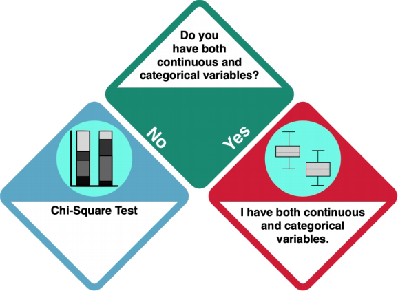
'''Your dataset does not only contain continuous data.''' Does it only consist of categorical data, or of categorical and continuous data? | '''Your dataset does not only contain continuous data.''' Does it only consist of categorical data, or of categorical and continuous data? | ||
<imagemap>Image:Statistics Flowchart - Data Formats.png|650px|center| | <imagemap>Image:Statistics Flowchart - Data Formats.png|650px|center| | ||
| − | poly | + | poly 288 2 151 139 289 271 424 138 [[Data formats]] |
| − | poly | + | poly 137 148 0 285 138 417 273 284 [[An_initial_path_towards_statistical_analysis#Only_categorical_data:_Chi_Square_Test|Only categorical data: Chi Square Test]] |
| − | poly | + | poly 436 151 299 288 437 420 572 287 [[An_initial_path_towards_statistical_analysis#Categorical_and_continuous_data|Categorical and continuous data]] |
</imagemap> | </imagemap> | ||
| Line 52: | Line 50: | ||
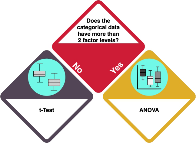
'''Your dataset consists of continuous and categorical data.''' How many levels does your categorical variable have? | '''Your dataset consists of continuous and categorical data.''' How many levels does your categorical variable have? | ||
<imagemap>Image:Statistics flowchart - Categorical factor levels.png|650px|center| | <imagemap>Image:Statistics flowchart - Categorical factor levels.png|650px|center| | ||
| − | poly | + | poly 321 3 175 149 325 304 473 152 473 15 [[An_initial_path_towards_statistical_analysis#Categorical_and_continuous_data]] |
| − | poly | + | poly 149 172 3 318 153 473 301 321 301 321 [[An_initial_path_towards_statistical_analysis#One_or_two_factor_levels: t-test|One or two factor levels: t-test]] |
| + | poly 489 172 343 318 493 473 641 321 641 321 [[An_initial_path_towards_statistical_analysis#More_than_two_factor_levels: ANOVA|More than two factor levels: ANOVA]] | ||
</imagemap> | </imagemap> | ||
| Line 67: | Line 66: | ||
<imagemap>Image:Statistics Flowchart - Equal variances.png|850px|center| | <imagemap>Image:Statistics Flowchart - Equal variances.png|850px|center| | ||
| − | poly | + | poly 146 5 0 150 145 290 289 148 [[Simple_Statistical_Tests#f-test|f-Test]] |
| − | poly | + | poly 557 2 408 147 556 286 700 144 [[Simple_Statistical_Tests#f-test|f-Test]] |
| − | poly | + | poly 392 165 243 310 391 450 535 308 [[Simple_Statistical_Tests#Most_relevant_simple_tests|t-Test]] |
| + | poly 716 160 567 305 715 444 859 302 [[Simple_Statistical_Tests#Most_relevant_simple_tests|t-Test]] | ||
</imagemap> | </imagemap> | ||
'''How do I know?''' | '''How do I know?''' | ||
| − | * Variance in the data is the measure of dispersion: how much the data spreads around the mean? Use an f-Test to check whether the variances of the two datasets are equal. The key R command for an f-test is <code>var.test()</code>. If the rest returns insignificant results, we can assume equal variances. Check the [[Simple_Statistical_Tests#f-test|f-Test]] entry to learn more. | + | * Variance in the data is the measure of dispersion: how much the data spreads around the mean? Use an f-Test to check whether the variances of the two datasets are equal. The key R command for an f-test is <code>var.test()</code>. If the rest returns insignificant results (>0.05), we can assume equal variances. Check the [[Simple_Statistical_Tests#f-test|f-Test]] entry to learn more. |
* If the variances of your two datasets are equal, you can do a Student's t-test. By default, the function <code>t.test()</code> in R assumes that variances differ, which would require a Welch t-test. To do a Student t-test instead, set <code>var.equal = TRUE</code>. | * If the variances of your two datasets are equal, you can do a Student's t-test. By default, the function <code>t.test()</code> in R assumes that variances differ, which would require a Welch t-test. To do a Student t-test instead, set <code>var.equal = TRUE</code>. | ||
==== More than two factor levels: ANOVA ==== | ==== More than two factor levels: ANOVA ==== | ||
| − | '''Your categorical variable has more than two factor levels: you | + | '''Your categorical variable has more than two factor levels: you are heading towards an ANOVA.'''<br/> |
| − | |||
| − | However, | + | '''However, you need to answer one more question''': what about the distribution of your dependent variable? |
<imagemap>Image:Statistics Flowchart - 2+ Factor Levels - normal distribution.png|650px|center| | <imagemap>Image:Statistics Flowchart - 2+ Factor Levels - normal distribution.png|650px|center| | ||
| − | poly | + | poly 291 5 150 140 291 270 423 136 [[Data distribution]] |
| − | poly | + | poly 141 152 0 287 141 417 273 283 261 270 [[ANOVA]] |
| − | poly | + | poly 442 152 301 287 442 417 574 283 562 270 [[ANOVA]] |
</imagemap> | </imagemap> | ||
'''How do I know?''' | '''How do I know?''' | ||
| − | * Inspect the data by looking at [[Introduction_to_statistical_figures#Histogram|histograms]]. The key R command for this is <code>hist()</code>. Compare your distribution to the [[Data distribution#Detecting_the_normal_distribution|Normal Distribution]]. | + | * Inspect the data by looking at [[Introduction_to_statistical_figures#Histogram|histograms]]. The key R command for this is <code>hist()</code>. Compare your distribution to the [[Data distribution#Detecting_the_normal_distribution|Normal Distribution]]. If the data sample size is big enough and the plots look quite symmetric, we can also assume it's normally distributed. |
| − | * | + | * You can also conduct the Shapiro-Wilk test, which helps you assess whether you have a normal distribution. Use <code>shapiro.test(data$column)</code>'. If it returns insignificant results (p-value > 0.05), your data is normally distributed. |
| + | |||
| + | Now, let us have another look at your variables. '''Do you have continuous and categorical independent variables?''' | ||
| + | |||
| + | '''How do I know?''' | ||
| + | * Investigate your data using <code>str</code> or <code>summary</code>. ''integer'' and ''numeric'' data is not ''categorical'', while ''factorial'', ''ordinal'' and ''character'' data is categorical. | ||
| + | |||
| + | If your answer is NO, you should stick to the ANOVA - more specifically, to the kind of ANOVA that you saw above (based on regression analysis, or based on a generalised linear model). An ANOVA compares the means of more than two groups by extending the restriction of the t-test. An ANOVA is typically visualised using [[Introduction_to_statistical_figures#Boxplot|Boxplots]].</br> The key R command is <code>aov()</code>. Check the entry on the [[ANOVA]] to learn more. | ||
| + | |||
| + | If your answer is YES, you are heading way below. Click [[An_initial_path_towards_statistical_analysis#Is_there_a_categorical_predictor?|HERE]]. | ||
| − | |||
| − | |||
== Only continuous variables == | == Only continuous variables == | ||
| Line 99: | Line 105: | ||
Now, you need to check if there dependencies between the variables. | Now, you need to check if there dependencies between the variables. | ||
<imagemap>Image:Statistics Flowchart - Continuous - Dependencies.png|650px|center| | <imagemap>Image:Statistics Flowchart - Continuous - Dependencies.png|650px|center| | ||
| − | poly | + | poly 383 5 203 181 380 359 559 182 [[Causality]] |
| − | poly | + | poly 182 205 2 381 179 559 358 382 [[An_initial_path_towards_statistical_analysis#No_dependencies:_Correlations|No dependencies]] |
| − | poly | + | poly 585 205 405 381 582 559 761 382 [[An_initial_path_towards_statistical_analysis#Clear_dependencies|Clear dependencies]] |
</imagemap> | </imagemap> | ||
| Line 115: | Line 121: | ||
<imagemap>Image:Statistics Flowchart - Normal Distribution.png|650px|center| | <imagemap>Image:Statistics Flowchart - Normal Distribution.png|650px|center| | ||
| − | poly | + | poly 288 3 154 137 289 269 421 136 [[Data distribution]] |
| − | poly | + | poly 135 151 1 285 136 417 268 284 268 284 [[Correlations|Pearson]] |
| + | poly 438 152 304 286 439 418 571 285 [[Correlations|Spearman]] | ||
</imagemap> | </imagemap> | ||
'''How do I know?''' | '''How do I know?''' | ||
| − | * Inspect the data by looking at [[Introduction_to_statistical_figures#Histogram|histograms]]. The key R command for this is <code>hist()</code>. Compare your distribution to the [[Data distribution#Detecting_the_normal_distribution|Normal Distribution]]. | + | * Inspect the data by looking at [[Introduction_to_statistical_figures#Histogram|histograms]]. The key R command for this is <code>hist()</code>. Compare your distribution to the [[Data distribution#Detecting_the_normal_distribution|Normal Distribution]]. If the data sample size is big enough and the plots look quite symmetric, we can also assume it's normally distributed. |
| − | * | + | * You can also conduct the Shapiro-Wilk test, which helps you assess whether you have a normal distribution. Use <code>shapiro.test(data$column)</code>'. If it returns insignificant results (p-value > 0.05), your data is normally distributed. |
| + | |||
=== Clear dependencies === | === Clear dependencies === | ||
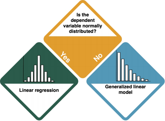
'''Your dependent variable is explained by one at least one independent variable.''' Is the dependent variable normally distributed? | '''Your dependent variable is explained by one at least one independent variable.''' Is the dependent variable normally distributed? | ||
<imagemap>Image:Statistics Flowchart - Dependent - Normal Distribution.png|650px|center| | <imagemap>Image:Statistics Flowchart - Dependent - Normal Distribution.png|650px|center| | ||
| − | poly | + | poly 289 2 152 139 290 267 423 13 [[Data distribution]] |
| − | poly | + | poly 137 151 0 288 138 416 271 281 [[An_initial_path_towards_statistical_analysis#Normally_distributed_dependent_variable:_Linear_Regression|Linear Regression]] |
| − | poly | + | poly 441 149 304 286 442 414 575 279 [[An_initial_path_towards_statistical_analysis#Not_normally_distributed_dependent_variable|Non-linear distribution of dependent variable]] |
</imagemap> | </imagemap> | ||
'''How do I know?''' | '''How do I know?''' | ||
| − | * Inspect the data by looking at [[Introduction_to_statistical_figures#Histogram|histograms]]. The key R command for this is <code>hist()</code>. Compare your distribution to the [[Data distribution#Detecting_the_normal_distribution|Normal Distribution]]. | + | * Inspect the data by looking at [[Introduction_to_statistical_figures#Histogram|histograms]]. The key R command for this is <code>hist()</code>. Compare your distribution to the [[Data distribution#Detecting_the_normal_distribution|Normal Distribution]]. If the data sample size is big enough and the plots look quite symmetric, we can also assume it's normally distributed. |
| − | * | + | * You can also conduct the Shapiro-Wilk test, which helps you assess whether you have a normal distribution. Use <code>shapiro.test(data$column)</code>'. If it returns insignificant results (p-value > 0.05), your data is normally distributed. |
| Line 146: | Line 154: | ||
'''You have several predictors (= independent variables) in your dataset.''' But is (at least) one of them categorical? | '''You have several predictors (= independent variables) in your dataset.''' But is (at least) one of them categorical? | ||
<imagemap>Image:Statistics Flowchart - Categorical predictor.png|650px|center| | <imagemap>Image:Statistics Flowchart - Categorical predictor.png|650px|center| | ||
| − | poly | + | poly 387 1 208 184 385 359 563 183 [[Data formats]] |
| − | poly | + | poly 180 197 1 380 178 555 356 379 [[An_initial_path_towards_statistical_analysis#ANCOVA|ANCOVA]] |
| − | poly | + | poly 584 196 405 379 582 554 760 378 [[An_initial_path_towards_statistical_analysis#Generalised_Linear_Models|Multiple Regression]] |
</imagemap> | </imagemap> | ||
| Line 163: | Line 171: | ||
'''The dependent variable(s) is/are not normally distributed.''' Which kind of distribution does it show, then? For both Binomial and Poisson distributions, your next step is the Generalised Linear Model. However, it is important that you select the proper distribution type in the GLM. | '''The dependent variable(s) is/are not normally distributed.''' Which kind of distribution does it show, then? For both Binomial and Poisson distributions, your next step is the Generalised Linear Model. However, it is important that you select the proper distribution type in the GLM. | ||
<imagemap>Image:Statistics Flowchart - Dependent - Distribution type.png|650px|center| | <imagemap>Image:Statistics Flowchart - Dependent - Distribution type.png|650px|center| | ||
| − | poly | + | poly 290 4 154 140 288 269 423 138 [[Data distribution]] |
| − | poly | + | poly 138 151 2 287 136 416 270 284 271 285 [[An_initial_path_towards_statistical_analysis#Generalised_Linear_Models|Generalised Linear Models]] |
| − | poly | + | poly 440 152 304 288 438 417 572 285 573 286 [[An_initial_path_towards_statistical_analysis#Generalised_Linear_Models|Generalised Linear Models]] |
</imagemap> | </imagemap> | ||
| Line 174: | Line 182: | ||
==== Generalised Linear Models ==== | ==== Generalised Linear Models ==== | ||
| − | '''You have arrived at a Generalised Linear Model (GLM).''' GLMs | + | '''You have arrived at a Generalised Linear Model (GLM).''' GLMs are a family of models that are a generalization of ordinary linear regressions. The key R command is <code>glm()</code>. |
Depending on the existence of random variables, there is a distinction between Mixed Effect Models, and Generalised Linear Models based on regressions. | Depending on the existence of random variables, there is a distinction between Mixed Effect Models, and Generalised Linear Models based on regressions. | ||
<imagemap>Image:Statistics Flowchart - GLM random variables.png|650px|center| | <imagemap>Image:Statistics Flowchart - GLM random variables.png|650px|center| | ||
| − | poly | + | poly 289 4 153 141 289 270 422 137 [[An_initial_path_towards_statistical_analysis#Generalised_Linear_Models]] |
| − | poly | + | poly 139 151 3 288 139 417 272 284 [[Mixed Effect Models]] |
| + | poly 439 149 303 286 439 415 572 282 [[Generalized Linear Models]] | ||
</imagemap> | </imagemap> | ||
'''How do I know?''' | '''How do I know?''' | ||
| − | * | + | * Random variables introduce extra variability to the model. For example, we want to explain the grades of students with the amount of time they spent studying. The only randomness we should get here is the sampling error. But these students study in different universities, and they themselves have different abilities to learn. These elements infer the randomness we would not like to know, and can be good examples of a random variable. If your data shows effects that you cannot influence but which you want to "rule out", the answer to this question is 'yes'. |
| + | |||
= Multivariate statistics = | = Multivariate statistics = | ||
| Line 191: | Line 201: | ||
Which kind of analysis do you want to conduct? | Which kind of analysis do you want to conduct? | ||
<imagemap>Image:Statistics Flowchart - Clustering, Networks, Ordination.png|center|650px| | <imagemap>Image:Statistics Flowchart - Clustering, Networks, Ordination.png|center|650px| | ||
| − | poly | + | poly 270 4 143 132 271 252 391 126 [[An_initial_path_towards_statistical_analysis#Multivariate_statistics]] |
| − | poly | + | poly 129 139 2 267 130 387 250 261 [[An_initial_path_towards_statistical_analysis#Ordinations|]] |
| − | poly | + | poly 407 141 280 269 408 389 528 263 [[An_initial_path_towards_statistical_analysis#Cluster_Analysis|]] |
| + | poly 269 273 142 401 270 521 390 395 [[An_initial_path_towards_statistical_analysis#Network_Analysis|]] | ||
</imagemap> | </imagemap> | ||
| Line 207: | Line 218: | ||
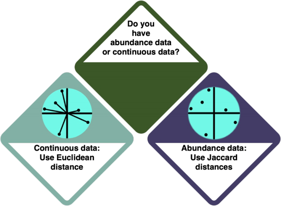
There is a difference between ordinations for different data types - for abundance data, you use Euclidean distances, and for continuous data, you use Jaccard distances. | There is a difference between ordinations for different data types - for abundance data, you use Euclidean distances, and for continuous data, you use Jaccard distances. | ||
<imagemap>Image:Statistics Flowchart - Ordination.png|650px|center| | <imagemap>Image:Statistics Flowchart - Ordination.png|650px|center| | ||
| − | poly | + | poly 288 6 153 141 289 268 419 137 [[Data formats]] |
| − | poly | + | poly 136 154 1 289 137 416 267 285 [[Big problems for later|Euclidean distances]] |
| − | poly | + | poly 439 149 304 284 440 411 570 280 [[Big problems for later|Jaccard distances]] |
</imagemap> | </imagemap> | ||
| Line 215: | Line 226: | ||
* Check the entry on [[Data formats]] to learn more about the different data formats. Abundance data is also referred to as 'discrete' data. | * Check the entry on [[Data formats]] to learn more about the different data formats. Abundance data is also referred to as 'discrete' data. | ||
* Investigate your data using <code>str</code> or <code>summary</code>. Abundance data is referred to as 'integer' in R, i.e. it exists in full numbers, and continuous data is 'numeric' - it has a comma. | * Investigate your data using <code>str</code> or <code>summary</code>. Abundance data is referred to as 'integer' in R, i.e. it exists in full numbers, and continuous data is 'numeric' - it has a comma. | ||
| − | + | ||
== Cluster Analysis == | == Cluster Analysis == | ||
| Line 222: | Line 233: | ||
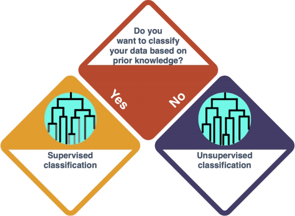
There is a difference to be made here, dependent on whether you want to classify the data based on prior knowledge (supervised, Classification) or not (unsupervised, Clustering). | There is a difference to be made here, dependent on whether you want to classify the data based on prior knowledge (supervised, Classification) or not (unsupervised, Clustering). | ||
<imagemap>Image:Statistics Flowchart - Cluster Analysis.png|650px|center| | <imagemap>Image:Statistics Flowchart - Cluster Analysis.png|650px|center| | ||
| − | poly | + | poly 290 3 157 138 289 270 421 134 [[Big problems for later|Classification]] |
| − | poly | + | poly 138 152 5 287 137 419 269 283 [[Clustering Methods]] |
| + | poly 437 153 304 288 436 420 568 284 [[Clustering Methods]] | ||
</imagemap> | </imagemap> | ||
'''How do I know?''' | '''How do I know?''' | ||
* Classification is performed when you have (X, y) pair of data (where X is a set of independent variables and y is the dependent variable). Hence, you can map each X to a y. Clustering is performed when you only have X in your dataset. So, this decision depends on the dataset that you have. | * Classification is performed when you have (X, y) pair of data (where X is a set of independent variables and y is the dependent variable). Hence, you can map each X to a y. Clustering is performed when you only have X in your dataset. So, this decision depends on the dataset that you have. | ||
| + | |||
== Network Analysis == | == Network Analysis == | ||
| Line 237: | Line 250: | ||
<imagemap>Image:Statistics Flowchart - Network Analysis.png|center|650px| | <imagemap>Image:Statistics Flowchart - Network Analysis.png|center|650px| | ||
| + | poly 290 5 155 137 289 270 419 134 [[An_initial_path_towards_statistical_analysis#Network_Analysis]] | ||
poly 336 364 4 684 340 1000 644 692 632 676 [[Big problems for later|Bipartite]] | poly 336 364 4 684 340 1000 644 692 632 676 [[Big problems for later|Bipartite]] | ||
poly 1064 372 732 700 1060 1008 1372 700 [[Big problems for later|Tripartite]] | poly 1064 372 732 700 1060 1008 1372 700 [[Big problems for later|Tripartite]] | ||
Latest revision as of 16:05, 12 December 2023
Learning statistics takes time, as it is mostly experience that allows us to be able to approach the statistical analysis of any given dataset. While we cannot take off of you the burden to gather experience yourself, we developed this interactive page for you to find the best statistical method to analyze your given dataset. This can be a start for you to dive deeper into statistical analysis, and helps you better design studies.
This page revolves around statistical analyses of data that has at least two variables. If you only have one variable, e.g. height data of a dozen trees, or your ratings for five types of cake, you might be interested in simpler forms of data analysis and visualisation. Have a look at Descriptive statistics and Introduction to statistical figures to see which approaches might work for your data.
If you have more than one variable, you have come to the perfect place!
Go through the images step by step, click on the answers that apply to your data, and let the page guide you.
If you need help with data visualisation for any of these approaches, please refer to the entry on Introduction to statistical figures.
If you are on mobile and/or just want a list of all entries, please refer to the Statistics overview page.
Start here with your data! This is your first question.
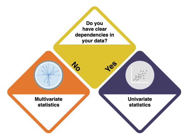

How do I know?
- What does the data show? Does the data logically suggest dependencies - a causal relation - between the variables? Have a look at the entry on Causality to learn more about causal relations and dependencies.
Contents
Univariate statistics
You are dealing with Univariate Statistics. Univariate statistics focuses on the analysis of one dependent variable and can contain multiple independent variables. But what kind of variables do you have?
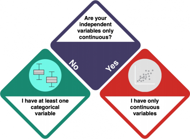

How do I know?
- Check the entry on Data formats to understand the difference between categorical and numeric (including continuous) variables.
- Investigate your data using
strorsummary. integer and numeric data is not categorical, while factorial, ordinal and character data is categorical.
At least one categorical variable
Your dataset does not only contain continuous data. Does it only consist of categorical data, or of categorical and continuous data?

How do I know?
- Investigate your data using
strorsummary. integer and numeric data is not categorical, while factorial, ordinal and character data is categorical.
Only categorical data: Chi Square Test
You should do a Chi Square Test.
A Chi Square test can be used to test if one variable influenced the other one, or if they occur independently from each other. The key R command here is: chisq.test(). Check the entry on Chi Square Tests to learn more.
Categorical and continuous data
Your dataset consists of continuous and categorical data. How many levels does your categorical variable have?

How do I know?
- A 'factor level' is a category in a categorical variable. For example, when your variable is 'car brands', and you have 'AUDI' and 'TESLA', you have two unique factor levels.
- Investigate your data using 'levels(categoricaldata)' and count the number of levels it returns. How many different categories does your categorical variable have? If your data is not in the 'factor' format, you can either convert it or use 'unique(yourCategoricalData)' to get a similar result.
One or two factor levels: t-test
With one or two factor levels, you should do a t-test.
A one-sample t-test allows for a comparison of a dataset with a specified value. However, if you have two datasets, you should do a two-sample t-test, which allows for a comparison of two different datasets or samples and tells you if the means of the two datasets differ significantly. The key R command for both types is t.test(). Check the entry on the t-Test to learn more.
Depending on the variances of your variables, the type of t-test differs.
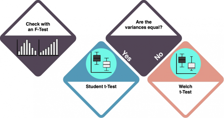

How do I know?
- Variance in the data is the measure of dispersion: how much the data spreads around the mean? Use an f-Test to check whether the variances of the two datasets are equal. The key R command for an f-test is
var.test(). If the rest returns insignificant results (>0.05), we can assume equal variances. Check the f-Test entry to learn more. - If the variances of your two datasets are equal, you can do a Student's t-test. By default, the function
t.test()in R assumes that variances differ, which would require a Welch t-test. To do a Student t-test instead, setvar.equal = TRUE.
More than two factor levels: ANOVA
Your categorical variable has more than two factor levels: you are heading towards an ANOVA.
However, you need to answer one more question: what about the distribution of your dependent variable?
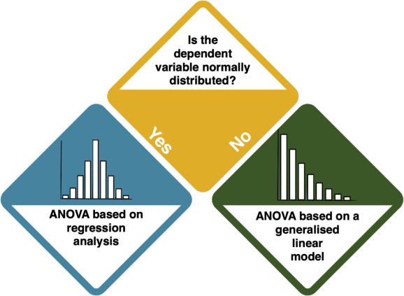

How do I know?
- Inspect the data by looking at histograms. The key R command for this is
hist(). Compare your distribution to the Normal Distribution. If the data sample size is big enough and the plots look quite symmetric, we can also assume it's normally distributed. - You can also conduct the Shapiro-Wilk test, which helps you assess whether you have a normal distribution. Use
shapiro.test(data$column)'. If it returns insignificant results (p-value > 0.05), your data is normally distributed.
Now, let us have another look at your variables. Do you have continuous and categorical independent variables?
How do I know?
- Investigate your data using
strorsummary. integer and numeric data is not categorical, while factorial, ordinal and character data is categorical.
If your answer is NO, you should stick to the ANOVA - more specifically, to the kind of ANOVA that you saw above (based on regression analysis, or based on a generalised linear model). An ANOVA compares the means of more than two groups by extending the restriction of the t-test. An ANOVA is typically visualised using Boxplots.
The key R command is aov(). Check the entry on the ANOVA to learn more.
If your answer is YES, you are heading way below. Click HERE.
Only continuous variables
So your data is only continuous.
Now, you need to check if there dependencies between the variables.

How do I know?
- Consider the data from a theoretical perspective. Is there a clear direction of the dependency? Does one variable cause the other? Check out the entry on Causality.
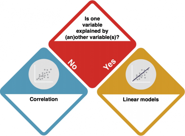
No dependencies: Correlations
If there are no dependencies between your variables, you should do a Correlation.
A correlation test inspects if two variables are related to each other. The direction of the connection (if or which variable influences another) is not set. Correlations are typically visualised using Scatter Plots or Line Charts. Key R commands are plot() to visualise your data, and cor.test() to check for correlations. Check the entry on Correlations to learn more.
The type of correlation that you need to do depends on your data distribution.
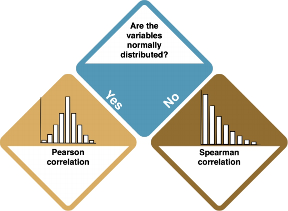

How do I know?
- Inspect the data by looking at histograms. The key R command for this is
hist(). Compare your distribution to the Normal Distribution. If the data sample size is big enough and the plots look quite symmetric, we can also assume it's normally distributed. - You can also conduct the Shapiro-Wilk test, which helps you assess whether you have a normal distribution. Use
shapiro.test(data$column)'. If it returns insignificant results (p-value > 0.05), your data is normally distributed.
Clear dependencies
Your dependent variable is explained by one at least one independent variable. Is the dependent variable normally distributed?

How do I know?
- Inspect the data by looking at histograms. The key R command for this is
hist(). Compare your distribution to the Normal Distribution. If the data sample size is big enough and the plots look quite symmetric, we can also assume it's normally distributed. - You can also conduct the Shapiro-Wilk test, which helps you assess whether you have a normal distribution. Use
shapiro.test(data$column)'. If it returns insignificant results (p-value > 0.05), your data is normally distributed.
Normally distributed dependent variable: Linear Regression
If your dependent variable(s) is/are normally distributed, you should do a Linear Regression.
A linear regression is a linear approach to modelling the relationship between one (simple regression) or more (multiple regression) independent and a dependent variable. It is basically a correlation with causal connections between the correlated variables. Check the entry on Regression Analysis to learn more.
There may be one exception to a plain linear regression: if you have several predictors (= independent variables), there is one more decision to make:
Is there a categorical predictor?
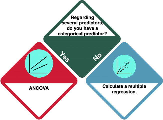
You have several predictors (= independent variables) in your dataset. But is (at least) one of them categorical?

How do I know?
- Check the entry on Data formats to understand the difference between categorical and numeric variables.
- Investigate your data using
strorsummary. Pay attention to the data format of your independent variable(s). integer and numeric data is not categorical, while factorial, ordinal and character data is categorical.
ANCOVA
If you have at least one categorical predictor, you should do an ANCOVA. An ANCOVA is a statistical test that compares the means of more than two groups by taking under the control the "noise" caused by covariate variable that is not of experimental interest. Check the entry on Ancova to learn more.
Not normally distributed dependent variable
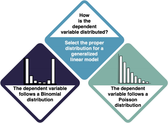
The dependent variable(s) is/are not normally distributed. Which kind of distribution does it show, then? For both Binomial and Poisson distributions, your next step is the Generalised Linear Model. However, it is important that you select the proper distribution type in the GLM.

How do I know?
- Try to understand the data type of your dependent variable and what it is measuring. For example, if your data is the answer to a yes/no (1/0) question, you should apply a GLM with a Binomial distribution. If it is count data (1, 2, 3, 4...), use a Poisson Distribution.
- Check the entry on Non-normal distributions to learn more.
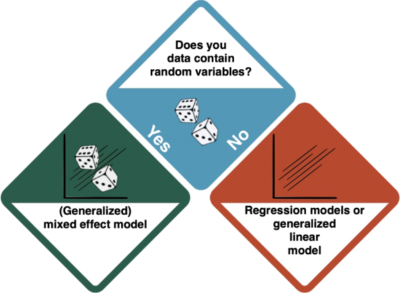
Generalised Linear Models
You have arrived at a Generalised Linear Model (GLM). GLMs are a family of models that are a generalization of ordinary linear regressions. The key R command is glm().
Depending on the existence of random variables, there is a distinction between Mixed Effect Models, and Generalised Linear Models based on regressions.

How do I know?
- Random variables introduce extra variability to the model. For example, we want to explain the grades of students with the amount of time they spent studying. The only randomness we should get here is the sampling error. But these students study in different universities, and they themselves have different abilities to learn. These elements infer the randomness we would not like to know, and can be good examples of a random variable. If your data shows effects that you cannot influence but which you want to "rule out", the answer to this question is 'yes'.
Multivariate statistics
You are dealing with Multivariate Statistics. Multivariate statistics focuses on the analysis of multiple variables at the same time.
Which kind of analysis do you want to conduct?
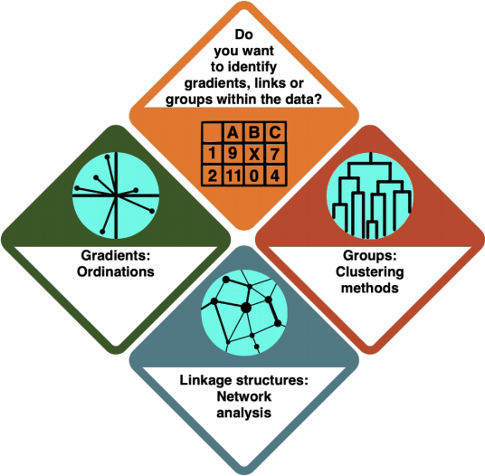

How do I know?
- In an Ordination, you arrange your data alongside underlying gradients in the variables to see which variables most strongly define the data points.
- In a Cluster Analysis (or general Classification), you group your data points according to how similar they are, resulting in a tree structure.
- In a Network Analysis, you arrange your data in a network structure to understand their connections and the distance between individual data points.
Ordinations
You are doing an ordination. In an Ordination, you arrange your data alongside underlying gradients in the variables to see which variables most strongly define the data points. Check the entry on Ordinations MISSING to learn more.
There is a difference between ordinations for different data types - for abundance data, you use Euclidean distances, and for continuous data, you use Jaccard distances.

How do I know?
- Check the entry on Data formats to learn more about the different data formats. Abundance data is also referred to as 'discrete' data.
- Investigate your data using
strorsummary. Abundance data is referred to as 'integer' in R, i.e. it exists in full numbers, and continuous data is 'numeric' - it has a comma.
Cluster Analysis
So you decided for a Cluster Analysis - or Classification in general. In this approach, you group your data points according to how similar they are, resulting in a tree structure. Check the entry on Clustering Methods to learn more.
There is a difference to be made here, dependent on whether you want to classify the data based on prior knowledge (supervised, Classification) or not (unsupervised, Clustering).

How do I know?
- Classification is performed when you have (X, y) pair of data (where X is a set of independent variables and y is the dependent variable). Hence, you can map each X to a y. Clustering is performed when you only have X in your dataset. So, this decision depends on the dataset that you have.
Network Analysis
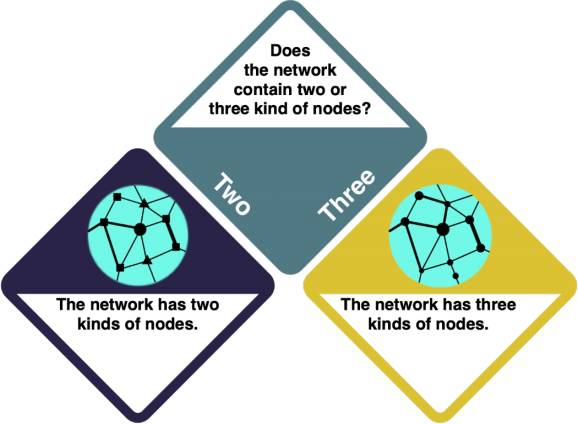
WORK IN PROGRESS You have decided to do a Network Analysis. In a Network Analysis, you arrange your data in a network structure to understand their connections and the distance between individual data points. Check the entry on Social Network Analysis and the R example entry MISSING to learn more. Keep in mind that network analysis is complex, and there is a wide range of possible approaches that you need to choose between.
How do I know what I want?
- Consider your research intent: are you more interested in the role of individual actors, or rather in the network structure as a whole?

Some general guidance on the use of statistics
While it is hard to boil statistics down into some very few important generalities, I try to give you here a final bucket list to consider when applying or reading statistics.
1) First of all, is the statistics the right approach to begin with? Statistics are quite established in science, and much information is available in a form that allows you to conduct statistics. However, will statistics be able to generate a piece of the puzzle you are looking at? Do you have an underlying theory that can be put into constructs that enable a statistical design? Or do you assume that a rather open research question can be approached through a broad inductive sampling? The publication landscape, experienced researchers as well as pre-test may shed light on the question whether statistics can contribute solving your problem.
2) What are the efforts you need to put into the initial data gathering? If you decided that statistics would be valuable to be applied, the question then would be, how? To rephrase this statement: How exactly? Your sampling with all its constructs, sample sizes and replicates decides about the fate of everything you going to do later. A flawed dataset or a small or biased sample will lead to failure, or even worse, wrong results. Play it safe in the beginning, do not try to overplay your hand. Slowly edge your way into the application of statistics, and always reflect with others about your sampling strategy.
3) The analysis then demands hand-on skills, as implementing tests within a software is something that you learn best through repetition and practice. I suggest you to team up with other peers who decide to go deeper into statistical analysis. If you however decide against that, try to find geeks that may help you with your data analysis. Modern research works in teams of complementary people, thus start to think in these dimensions. If you chip in the topical expertise of the effort to do the sampling, other people may be glad about the chance to analyse the data.
4) This is also true for the interpretation, which most of all builds on experience. This is the point were a supervisor or a PhD student may be able to glance at a result and tell you which points are relevant, and which are negotiable. Empirical research typically produces results where in my experience about 80 % are next to negliable. It takes time to learn the difference between a trivial and an innovative result. Building on knowledge of the literature helps again to this end, but be patient as the interpretation of statistics is a skill that needs to ripen, since context matters. It is not so much about the result itself, but more about the whole context it is embedded in.
5) The last and most important point explores this thought further. What are the limitations of your results? Where can you see flaws, and how does the multiverse of biases influence your results and interpretation? What are steps to be taken in future research? And what would we change if we could start over and do the whole thing again? All these questions are like ghosts that repeatedly come to haunt a researcher, which is why we need to remember we look at pieces of the puzzle. Acknowledging this is I think very important, as much of the negative connotation statistics often attracts is rooted in a lack of understanding. If people would have the privilege to learn about statistics, they could learn about the power of statistics, as wells its limitations.
Never before did more people in the world have the chance to study statistics. While of course statistics can only offer a part of the puzzle, I would still dare to say that this is reason for hope. If more people can learn to unlock this knowledge, we might be able to move out of ignorance and more towards knowledge. I think it would be very helpful if in a controversial debate everybody could dig deep into the available information, and make up their own mind, without other people telling them what to believe. Learning about statistics is like learning about anything else, it is lifelong learning. I believe that true masters never achieve mastership, instead they never stop to thrive for it.
The authors of this entry are Henrik von Wehrden (concept, text) and Christopher Franz (implementation, linkages).