Difference between revisions of "Regression Analysis"
| (One intermediate revision by one other user not shown) | |||
| Line 1: | Line 1: | ||
| − | [[File: | + | [[File:Quan dedu indi syst glob past pres futu.png|thumb|right|[[Design Criteria of Methods|Method Categorisation:]]<br> |
| − | <br | + | '''Quantitative''' - Qualitative<br> |
| − | + | '''Deductive''' - Inductive<br> | |
| − | + | '''Individual''' - '''System''' - '''Global'''<br> | |
| − | + | '''Past''' - '''Present''' - '''Future''']] | |
| − | |||
| − | |||
| − | |||
| − | |||
| − | |||
| − | |||
| − | |||
| − | |||
| − | |||
| − | |||
'''In short:''' Regression analysis tests whether a relation between two continuous variables is positive or negative, how strong the relation is, and whether the relation is significantly different from chance. | '''In short:''' Regression analysis tests whether a relation between two continuous variables is positive or negative, how strong the relation is, and whether the relation is significantly different from chance. | ||
<br/> | <br/> | ||
| Line 19: | Line 9: | ||
'''Note:''' This entry revolves around simple linear regressions and the fundamentals of regression analysis. For more info, please refer to the entries on [[Causality and correlation]] as well as [[Generalized Linear Models]]. | '''Note:''' This entry revolves around simple linear regressions and the fundamentals of regression analysis. For more info, please refer to the entries on [[Causality and correlation]] as well as [[Generalized Linear Models]]. | ||
| + | __TOC__ | ||
== Background == | == Background == | ||
Latest revision as of 12:00, 18 March 2024
Quantitative - Qualitative
Deductive - Inductive
Individual - System - Global
Past - Present - Future
In short: Regression analysis tests whether a relation between two continuous variables is positive or negative, how strong the relation is, and whether the relation is significantly different from chance.
Note: This entry revolves around simple linear regressions and the fundamentals of regression analysis. For more info, please refer to the entries on Causality and correlation as well as Generalized Linear Models.
Contents
Background
The question whether two continuous variables are linked initially emerged with the rise of data from astronomical observation. Initial theoretical foundations were laid by Gauss and Legendre, yet many relevant developments also happened much later. At their core, the basics of regressions revolved around the importance of the normal distribution. While Yule and Pearson were more rigid in recognising the foundational importance of the normal distribution of the data, Fisher argued that only the response variable needs to follow this distribution. This highlights yet another feud between the two early key innovators in statistics - Fisher and Pearson - who seem to be only able to agree to disagree on each other. The regression analysis was rooted famously in an observation by Galton called regression towards the mean - which proclaims that within most statistical samples, an outlier point is more likely than not followed by a data point that is closer to the mean. This proves to be a natural law for many dynamics that can be observed, underlining the foundational importance of the normal distribution, and how it translates into our understanding of patterns in the world.
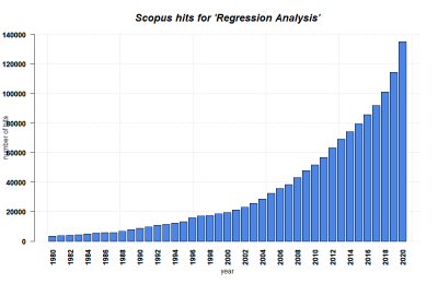
Regressions rose to worldwide recognition through econometrics, which used the increasing wealth of data from nation states and other systems to find relations within market dynamics and others patterns associated to economics. Equally, the regression was increasingly applied in medicine, engineering and many other fields of science. The 20th century became a time ruled by numbers, and the regression was one of its most important methods. Today, it is commonplace in all branches of science that utilise quantitative data to analyze data through regressions, including economics, social science, ecology, engineering, medicine, psychology, and many other branches of science. Almost all statistical software packages allow for the analysis of regressions, the most common software solutions are R, SPSS, Matlab and Python. Thanks to the computer revolutions, most regressions are easy and fast in their computation, and with the rising availability of more and more data, the regression became the most abundantly used simple statistical model that exists to date.
What the method does
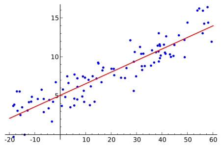
Regressions statistically test the dependence of one continuous variable with another continuous variable. Building on a calculation that resolves around least squares, regression analysis can test whether a relation between to continuous variables is positive or negative, how strong the relation is, and whether the relation is significantly different from chance, i.e. following a non-random pattern. This is an important difference to Correlations, which only revolve around the relation between variables without assuming - or testing for - a causal link. Thus, identifying regressions can help us infer predictions about future developments of a relation.
Within a regression analysis, a dependent variable is explained by an independent variable, both of which are continuous. At the heart of any regression analysis is the optimisation of a regression line that minimises the distance of the line to all individual points. In other words, the least square calculation maximizes the way how the regression line can integrate the sum of the squares of all individual data points to the regression line. The line can thus indicate a negative or positive relation by a negative or positive estimate, which is the value that indicates how much the y value increases if the x value increases.
The sum of the squares of the distance of all points to the regression line allows to calculate an r squared value. It indicates how strong the relation between the x and the y variable is. This value can range from 0 to 1, with 0 indicating no relation at all, and 1 indicating a perfect relation. There are many diverse suggestions of what constitutes a strong or a weak regression, and this depends strongly on the context.
Lastly, the non-randomness of the relation is indicated by the p-value, which shows whether the relation of the two continuous variables is random or not. If the p-value is below 0,05 (typically), we call the relation significant. If there is a significant relation between the dependent and the independent variable, then new additional data is supposed to follow the same relation (see 'Prediction' bevlow). There are diverse ideas whether the two variables should follow a normal distribution, but it is commonly assumed that if the residuals - which is the deviation of the data points from a perfect relation - should follow a normal distribution. In other words, the error that is revealed through your understanding of the observed pattern follows a statistical normal distribution. Any non-normally distributed pattern might reveal flaws in sampling, a lack of additional variables, confounding factors, or other profound problems that limit the value of your analysis.
Probability
Probability is one of the most important concepts in modern statistics. The question whether a relation between two variables is purely by chance, or following a pattern with a certain probability, is the basis of all probability statistics (surprise!). In the case of linear relations, another quantification is of central relevance: the question how much variance is explained by the model. These two things - the amount of variance explained by a linear model, and the fact that two variables are not randomly related - are related at least to some amount. If a model is highly significant, it typically shows a high r squared value. If a model is marginally significant, then the r squared value is typically low.
This relation is however also influenced by the sample size. Linear models and the related p-value describing the model are highly sensitive to sample size. You need at least a handful of points to get a significant relation, even if the r squared value in this model with a small sample size may be already high. Therefore, the relation between sample size, the r squared value and the p-value is central to understand how meaningful a model is.
Prediction
Regression analysis may allow for predictions based on available data. Predictions are a common element of statistics. In general, prediction means that we are able to foresee data beyond the range of our available data, based on the statistical power of our model which we developed based on the available data. In other words, we have enough confidence in our initial data analysis so that we can try to predict what might happen under other circumstances. Most prominently, people predict data in the future, or in other places, which is called extrapolation. By comparison, interpolation allows us to predict within the range of our data, spanning over gaps in the data. Hence while interpolation allows us to predict within our data, extrapolation allows prediction beyond our dataset.
Care is necessary when considering interpolation or extrapolation, as validity decreases when we dwell beyond the data we have. It takes experience to know when prediction is possible, and when it is dangerous.
- We need to consider if our theoretical assumptions can be reasonable expanded beyond the data of our sample.
- Our statistical model may be less applicable outside or our data range.
- Mitigating or interacting factors may become more relevant in the space outside of our sample range.
We always need to consider these potential flaws or sources of error that may overall reduce the validity of our model when we use it for interpolation or extrapolation. As soon as we gather outside of the data space we sampled, we take the risk to produce invalid predictions. The "missing shade of blue" problem from Hume exemplifies the ambiguities that can be associated with interpolation already, and extrapolation would be seen as worse by many, as we go beyond our data sample space.
A common example of extrapolation would be a mechanistic model of climate change, where based on the trend in CO2 rates on Mauna Loa over the last decades we predict future trends. A prominent example of interpolation is the Worldclim dataset, which generates a global climate dataset based on advanced interpolation. Based on ten thousands of climate stations and millions of records this dataset provides knowledge about the average temperature and precipitation of the whole terrestrial globe. The data has been used in thousands of scientific publications and is a good example of how open source data substantially enabled a new scientific arena, namely Macroecology.
Regressions, in comparison, are rather simple models which may still allow us to predict data. If our regression shows a significant relation between two variables, and is able to explain a major part of the variance, we can use the regression for extra- or interpolation - while respecting the limitations mentioned above.
Strengths & Challenges
Causality
The main strength of regressions is equally their main weakness: Regression analysis examines the dependence of one continuous variable on another continuous variable. Consequently, this may be either describing a causal pattern or not. The question of causality in regression can be extremely helpful if examined with care. More information on causality can be found here. The main points to consider are the criteria of Hume: If A causes B, then A has a characteristic that leads to B. If C does not lead to B, then C has a characteristic that differs from A. Also, causality is build on temporal sequence: only if A happens before B, then A can lead to B. All this is relevant for regressions, as the dependence between variables may be interpreted as causality.
The strongest point of regression models may be that we can test hypotheses, yet this poses also a great danger, because regressions can be applied both inductively and deductively. A safe rooting in theory seems necessary in order to test for meaningful relationships between to variables.
Regression analysis builds on p-values, and many people utilising regression analysis are next to obsessed with high r squared values. However, the calculation of p-values can be problematic due to statistical fishing: the more models are calculated, the higher the chance to find something significant. Equally difficult is the orientation along r squared values. There is no universally agreed threshold that differentiates a good from a bad model, instead the context matters. As usual, different conventions and norms in the diverse branches of science create misunderstandings and tensions
Data distribution
Regressions strongly resolve around the normal distribution. While many phenomena that can be measured meet this criteria, the regression fails with much of the available datasets that consist of count (or 'discrete') data. Other distributions are incorporated into more advanced methods of analysis, such as generalised linear models, and we have to acknowledge that the regression works robustly for normally distributed data, but only for these datasets where this criteria is met.
Taken together, it can be concluded that the regression is one of the most simple and robust model available in statistics, yet the world moved on and spawned more complex models that are better able to take more diverse assumptions into account. The regression is still suitable for the original case for which it was proposed, testing the dependence between two continuous variables, and building on an understanding of such derived patterns that widely resolves around the normal distribution.
Normativity
The main problem for regression analysis is that these models are applied in cases that do not meet the necessary assumptions. Many problems that were derived from regressions models surfaced because users ignored the original assumptions resolving around normal distributions, or tried to press patterns into a linear line of thinking that does not meet the reality of the data. Regressions can be seen as a main tool that led to the failure of positivism, because regressions always analyse a snapshot in time, and dynamics of data may change. The financial crisis is a good example, where on one day all patterns deviated from the previous pattern that were analysed by most stock brokers, thereby triggering a cascade of effects and patterns that can be predicted by regression models, but only at a dramatically different time horizon. While before, market shifts operated on a scale of months, shifts in the market suddenly came to be in a matter of seconds. Both patterns can be explained by regressions, but the temporal horizon of the analysis makes them almost incomparable. Such effects can be described as phase shifts, and the standard regression is not able to meaningfully combine such changes into one model.
An equally challenging situation can be diagnosed for spatial scales. Econometrics can be able to generate predictions about market shifts at a global scale, but less can be said how an individual business operating at a much smaller scale will be affected. Regression model can be operationalised at one spatial scale, but these models cannot be easily upscaled to a different scale. If I measure the growth of biomass at a plant scale, it would be hard to upscale any assumptions based on these measurements and models of individual plants to a global scale. If I did, I would assume that the conditions at the specific spots where I measure are the same across the globe - which is rarely the case. Regressions are thus very robust at the spatial scale at which they are operationalised, but often can say very little beyond that scale.
What is more, regressions are typically showing you a certain linear dependence that has an underlying variance. Especially in the public debate and its understanding of statistics, this is often overseen. Very often, people assume that a relation revealed by a regression is a very tamed relation. Instead, most regressions show a high variance, making predictions of future data vague. Many medical breakthroughs discuss matters that are based on models that explain less than half of the variance in the available data. In other words, many data points do not strongly follow this pattern, but instead show a high deviance - which we cannot explain. This creates a strong notion that statistics, or even statisticians, are lying. While this is certainly an overly bold conclusion, we can indeed pinpoint many examples where scientists discuss patterns as if they were very precise, although they are not.
This is one of the main fallacies of positivistic science. Not only are their fundamental assumptions about the objectivity of knowledge wrong, but positivists often fail to highlight the limitations of their knowledge. In the case of regressions, this would be the variance, and the less-than-perfect sum of squares that can highlight how much the model explains. This failure to highlight the limitations of a model is nowhere more drastic than in the complex statistics that are behind the word 'significance'. A significant relation is a non-random relation, indicating a pattern that cannot be associated to chance. More often than not, however, this says very little about the strength of the relation. On the contrary, for almost all but a small number cases, regressions that are significant not necessarily respresent strong relations. Instead, many significant relations can be quite weak, with an explained r squared of 0.13 already being significant in large case examples. In other words, the vast majority of the relation is unexplained. This would be perfectly alright if we understood it in this way, and indicate the abilities of the model. With the rise of soft science and its utilisation of statistics, however, this limitation of statistical analysis is often overseen when it comes to the public debate of statistical relations, and their relevance for policy decisions.
Yet there are also direct limitations or reasons for concern within science itself. Regressions were initially derived to test for dependence between two continuous variables. In other words, a regression is at its heart a mostly deductive approach. This has been slowly eroded over the last decades, and these days many people conduct regression analysis that do not test for statistical fishing, and end up being just that. If we test long enough for significant relations, there will eventually be one, somewhere in the data. It is however tricky to draw a line, and many of the problems of the reproducibility crisis and other shortcomings of modern sincere can be associated to the blur if not wrong usage of statistical models.
The last problem of regression analysis is the diversity of disciplinary norms and conventions when it comes to the reduction of complex models. Many regressions are multiple regressions, where the dependent variable is explained by many predictors (= independent variables). The interplay and single value of several predictors merits a model reduction approach, or alternatively a clear procedure in terms of model constructions. Different disciplines, but also smaller branches of sciences, differ vastly when it comes to these diversities, making the identification of the most parsimonious approach currently a challenge.
Simple linear regression in R
As mentioned before, R can be a powerful tool for visualising and analysing regressions. In this section we will look at a simple linear regression using "forbes" dataset.
First of all we need to load all the packages. In this example, we will use the forbes dataset from the library MASS.
install.packages("MASS", repos = "ttp://cran.us.r-project.org")
library(tidyverse)
library(MASS)

#Let's look closer at the dataset
?forbes
We can see that it is a dataframe with 17 observations corresponding to observed boiling point and corrected barometric pressure in the Alps. Let's arrange the dataset and convert it into a tibble in order to make it easier to analyze. It allows us to manipulate the dataset quickly (because the variables type is directly displayed).
forbes_df <- forbes   # We just rename the data
forbes_tib <- as_tibble(forbes_df) # Convert the dataframe into a tibble
head(forbes_tib)     # Shows first 6 rows of dataset

#Output:
## # A tibble: 6 x 2
##      bp  pres
##   <dbl> <dbl>
## 1  194.  20.8
## 2  194.  20.8
## 3  198.  22.4
## 4  198.  22.7
## 5  199.  23.2
## 6  200.  23.4

str(forbes_tib)     # Structure of Prestige dataset

#Output:
## Classes 'tbl_df', 'tbl' and 'data.frame':    17 obs. of  2 variables:
##  $ bp  : num  194 194 198 198 199 ...
##  $ pres: num  20.8 20.8 22.4 22.7 23.1 ...
It is important to be sure that there is no missing value ("NA") to apply the linear regression. In case of the forbes dataset, which is basically small, we can see that there is no NA.
summary(forbes_tib)  # Summarize the data of forbes

#Output:
##        bp             pres
##  Min.   :194.3   Min.   :20.79
##  1st Qu.:199.4   1st Qu.:23.15
##  Median :201.3   Median :24.01
##  Mean   :203.0   Mean   :25.06
##  3rd Qu.:208.6   3rd Qu.:27.76
##  Max.   :212.2   Max.   :30.06
In order to make it easier to understand for us, we are going to convert the two variables: 1. the boiling temperature of the water (From Farenheit to Celcius). We will use the formula to convert a temperature from Farenheit to Celcius: C = 5/9 x (F-32)
require(MASS)
require(dplyr)
FA <- forbes_tib %>%  # We define a table F that stands for the F in the above formula
  dplyr::select(bp)  # and containing all the information concerning Temperatures

TempCel <- ((5/9) * (FA-32))
TempCel

#Output:
##           bp
## 1   90.27778
## 2   90.16667
## 3   92.16667
## 4   92.44444
## 5   93.00000
## 6   93.27778
## 7   93.83333
## 8   93.94444
## 9   94.11111
## 10  94.05556
## 11  95.33333
## 12  95.88889
## 13  98.61111
## 14  98.11111
## 15  99.27778
## 16  99.94444
## 17 100.11111
2. the barometric pressure (From inches of mercury to hPa). We will use the following formula to convert inches of mercury: hPa = Pressure (inHg) x 33.86389
require(MASS)
require(dplyr)
Press1 <- forbes_tib %>%
  dplyr::select(pres)


PressureHpa <- Press1 * 33.86389
PressureHpa

## Output:
##         pres
## 1   704.0303
## 2   704.0303
## 3   758.5511
## 4   767.6944
## 5   783.9491
## 6   790.7218
## 7   809.0083
## 8   812.3947
## 9   813.4106
## 10  813.0720
## 11  851.3382
## 12  899.7636
## 13  964.7822
## 14  940.0616
## 15  983.4074
## 16 1011.8530
## 17 1017.9485
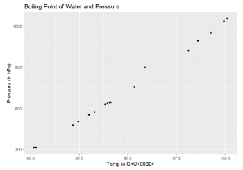
Let's save a new dataframe with the converted values. We will use a Scatter Plot to visualise if there is a relationship between the variables (so we can apply the linear regression). Scatter Plots can help visualise linear relationships between the response and predictor variables. The purpose here is to build an equation for pressure as a function of temperature: to predict pressure when only the temperature (boiling point) is known.
# Saving and viewing the new dataframe
BoilingPoint <- data.frame(TempCe=TempCel,PressureHpa=PressureHpa)
View(BoilingPoint)
# Visualising
# Fig.1
ggplot(BoilingPoint, aes(x = bp , y = pres)) + geom_point() +
xlab ("Temp in Cæ¼ã¸°") + ylab("Pressure (in hPa)") +
ggtitle ("Boiling Point of Water and Pressure")
The scatter Plot suggest here a linear relationship between the temperature and the pressure.In this case, Pressure is the dependant variable ('target variable').
cor(BoilingPoint$bp,BoilingPoint$pres)

## Output:
## [1] 0.9972102
We compute the correlation coefficient in order to see the degree of linear dependence between temp and pres. The value of 0.9972102 is close to 1 so they have a strong positive correlation. To remember: Correlation can only take values between -1 and + 1.
# Fig.2
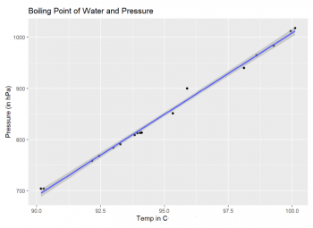
ggplot(BoilingPoint, aes(x = bp , y =  pres)) +  geom_point() +
xlab ("Temp in C°") + ylab("Pressure (in hPa)") +
ggtitle ("Boiling Point of Water and Pressure") + geom_smooth(method="lm")

#Building linear model
PressTempModel <- lm(pres ~ bp, data = BoilingPoint)
print(PressTempModel)

## Output
##
## Call:
## lm(formula = pres ~ bp, data = BoilingPoint)
##
## Coefficients:
## (Intercept)           bp
##    -2178.50        31.87
We successfully established the linear regression model. It means that we built the relationship between the predictor (Temp) and response variables (Pressure) <- taking form of a formula:
- Pressure = - 2178.5 + (31.87*temperature)
- Pressure = Intercept + (Beta coefficient of temperature*temperature)
It will allow us to predict pressure values with temperature values.
summary(PressTempModel)

## Output:
##
## Call:
## lm(formula = pres ~ bp, data = BoilingPoint)
##
## Residuals:
##    Min     1Q Median     3Q    Max
## -8.709 -3.808 -1.728  4.837 22.010
##
## Coefficients:
##              Estimate Std. Error t value Pr(>|t|)
## (Intercept) -2178.504     58.536  -37.22 3.41e-16 ***
## bp             31.873      0.616   51.74  < 2e-16 ***
## ---
## Signif. codes:  0 '***' 0.001 '**' 0.01 '*' 0.05 '.' 0.1 ' ' 1
##
## Residual standard error: 7.885 on 15 degrees of freedom
## Multiple R-squared:  0.9944, Adjusted R-squared:  0.9941
## F-statistic:  2677 on 1 and 15 DF,  p-value: < 2.2e-16
- "P Value: < 2.2e-16" – effectively close to zero meaning we reject the null hypothesis (co-efficient of the predictor is zero), i.e. the model is statistically significant. Our p-value is < than the statistical significance level of 0.05. 0.05 can be compared as a threshold.
- Residuals here can be considered as the distance from the data points to the line.
- In our case, the t-value (in absolute value) is high, meaning our p-value will be small.
- Multiple R-squared (0.9944) and adjusted R-squared (0.9941) show how well the model fits our data. We use R-Squared to measure how close each of our datapoints fits to the regression line. This measure is always between 0 and 1 (or 0% and 100%). We can say that the larger the R², the better the model fits your observations. In our case, the R² value is > 0.99, meaning our model fits our observations very well.
Outlook
Regression models are rather limited in their assumptions, building on the normal distribution, and being unable to implement more complex design features such as random intercepts or random factors. While regressions surely serve as the main basis of frequentist statistics, they are mostly a basis for more advanced models these days, and seem almost outdated compared to the wider available canon of statistics. To this end, regressions can be seen as a testimony that the reign of positivism needs to come to an end. Regressions can be powerful and robust, but regressions are equally static and simplistic. Without a critical perspective and a clear recognition of their limitations, we may exceed the value of regressions beyond their capabilities.
The question of model reduction will preoccupy statistics for the next decades, and this development will be interacting with a further rise of Bayes theorem and other questions related to information processing. Time will tell how regressions will emerge on the other side, yet it is undeniable that there is a use case for this specific type of statistical model. Whether science will become better in terms of the theoretical foundations of regressions, in recognising and communicating the restrictions and flaws of regressions, and not overplaying their hand when it comes to the creation of knowledge, is an altogether different story.
Key Publications
References
The authors of this entry are Henrik von Wehrden and Quentin Lehrer.
