Partial Correlation

Note: This entry revolves specifically around Partial Correlations. For more general information on quantitative data visualisation, please refer to Introduction to statistical figures. For more info on Data distributions, please refer to the entry on Data distribution.

In short: Partial Correlation is a method to measure the degree of association between two variables, while controlling for the impact, a third variable has on both. When looking at correlations, they can often be misleading and must be treated with care. For example, this website provides a list of strongly significant correlations that do not seem to have a meaningful and direct connection. This undermines that correlation is not necessarily related to causality. On the one hand, this may be due to the principle of null hypothesis testing (see p-value). But in the case of correlation, strong significances can often be caused by a relationship to a common third variable and are therefore biased.

Problem Set

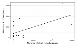
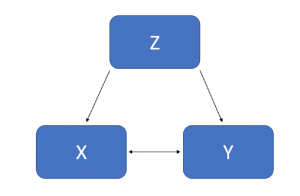
Fig.1: Stock populations and human birth across Europe. From Matthews (2001).

Fig.2: Model of partial correlations.

Let's consider this example from Matthews (2001) on stork populations and human birth rates across Europe (Fig.1). A correlation between both variables indicates a statistically significant positive relation of r = .62. But can we really make sense of this correlation? Does it mean that storks deliver babies? It is very likely that the connection can be explained by one (or more) external variable(s), for example by how rural the area of measurement is (see Figure 2). In a more rural area, more children are born and at the same time there is more space for storks to build their nests. So how can we control for this effect in a correlation analysis?

Assumptions

To use partial correlation and gain valid results, some assumptions must be fulfilled. No worries if these assumptions are violated! There is often still a work-around that can be done to bypass them.

Both variables and the third variable to control for (also known as control variable or covariate) must be measured on a continuous scale.
There needs to be a linear relationship between all three variables. This can be inspected by plotting every possible pair of variables.
There should be no significant outliers. Partial correlation is sensitive to outliers, because they have a large effect on the regression and correlation coefficients. Determining if a point is really a significant outlier, is most likely based on personal experience and can therefore be ambiguous
All variables should be approximately normally distributed.

Notion of Partial Correlation

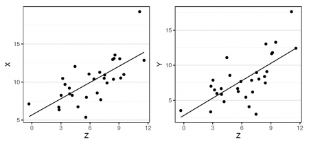
To check if a connection between two variables is caused by a common third variable, we test whether the relationship still exists after we have accounted for the influence of the third variable. This can be achieved by calculating two simple [Regression Analysis|linear regressions] to predict each of the two variables based on the expected third variable. Thus, we account for the impact the third variable has on the variance of each of our two variables.

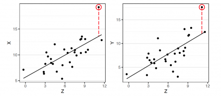
That way we can now consider the left-over (unexplained) variance - namely the residuals of the regressions. To better understand, why we are doing this, let s look at an individual data point of the regressions. If this point exceeds the predictions for both regressions equally, then there seems to be a remaining connection between both variables. So, when looking back at the broad picture of every data point, this means that if the residuals of both regressions are unrelated, then the relationship of the two variables could be explained by the third variable.

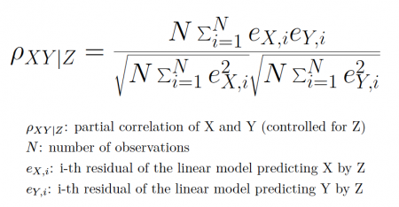
So in conclusion, to control for the impact of a third variable, we calculate the correlation between the residuals resulting from the two linear regressions of the variables with respect to the third variable. The resulting formula for partial correlation is:

It is also possible to add more than one control variable. We then use another, recursive formula. However, it is not recommended to add more than 2 control variables, because more variables impair the reliability of the test and the complexity of the recursive algorithm increases exponentially. When checking for the “unbiased” effect of multiple variables, it might be better to use a multiple linear regression instead.

Partial Correlation vs. Multiple Linear Regression

When thinking about partial correlation, one might notice that the basic idea is similar to a multiple linear regression. Even though a correlation is bidirectional while a regression aims at explaining one variable by another, in both approaches we try to identify the true and unbiased relationship of two variables. So when should we use which method? In general, partial correlation is a building step for multiple linear regression. Accordingly, linear regression has a broader range of applications and is therefore in most cases the method to choose. Using a linear regression, one can model interaction terms and it is also possible to loosen some assumptions by using a generalized linear model. Nevertheless, one advantage, partial correlation has over linear regression, is that it delivers an estimate for the relationship which is easy to interpret. The linear regression outputs weights that depend on the unit of measurement, making it hard to compare them to other models. As a work-around, one could use standardized beta coefficients. Yet those coefficients are harder to interpret since they do not necessarily have an upper bound. Partial correlation coefficients, on the other hand, are defined to range from -1 to 1.

Example for Partial Correlation using R

Partial Correlation can be performed using R. Let s consider the following (fictitious) data. The capital of the following sample of workers is correlated to the number of annual doctor visits (r ≈ .895).

# Fig.3
df <- data.frame(doctor_visits, capital, age)

Fig.3: "doctor_visits" data frame.

One way to perform a partial correlation on this data is to manually calculate it.

# First, we calculate the 2 simple linear regressions
model1 <- lm(doctor_visits~age)
model2 <- lm(capital~age)
# Next, we save the residuals of both linear models
res1 <- model1$residuals
res2 <- model2$residuals
# Finally, we can calculate the partial correlation by correlating the residuals
cor(res1, res2)

## Output:
## [1] 0.08214041

However, there are also a lot of pre-build packages for calculating a partial correlation. They provide an easier use and are especially more convenient when controlling for more than one variable. One example is the package ppcor.

Fig.4: Partial-correlation matrix

if (!require(ppcor)) install.packages('ppcor')
library(ppcor)
# The function generates a partial-correlation-matrix of every variable in the data frame!
# Fig.4
pcor(df)$estimate

We can see that the result for doctor visits and capital is identical to our manual approach.

The author of this entry is Daniel Schrader.