Price Determinants of Airbnb Accommodations

In short: This entry represents an analysis of airbnb data, starting from data scraping and analysis, to training and creating a machine learning model for price prediction. In this entry you will learn how to prepare and explore data, perform data cleaning, build wordmaps, choropleth maps, boxplots and scatterplots, as well as extract features and train a machine learning model.

Note: For more general information on quantitative data visualisation, please refer to Introduction to statistical figures. For more info on Data distributions, please refer to the entry on Data distribution.

Introduction

Knowing the market value of an overnight stay in an Airbnb home is of high interest for both, renters (or hosts) and guests. As a guest one might be a bit overwhelmed going through all the offers Airbnb nowadays contains (approximately 51.000 for the city of New York as of November 2018). Knowing exactly what drives prices of Airbnb listings could make the whole search process more enjoyable. Setting the right price on the other hand is a crucial tasks for the hosts, as they want neither, their listing not being booked, nor to rent it out too cheap.

To tackle these problems, this report aims at identifying the determinants of prices for Airbnb listings. More precisely, the following questions will be answered throughout the analysis:

1. How do hosts promote their listing? How are expensive/cheap listings being promoted?
2. What areas are the most expensive ones? Does this correlate with the location score?
3. Are there any seasonal effects on the price?
4. What are the overall most important determinants for the price?

The data

Data description

Airbnb itself does only provide a very limited insight into their data, but a separate group named Inside Airbnb scrapes and compiles publicly available information about many cities' listings from the Airbnb website. For this report, data for the city of New York from the year 2018 was been analysed. The dataset can be accessed through this link. Otherwise, more up-to-date datasets from the same website can be used for this analysis, making sure the features described and used for it appear in the tables.

The current dataset comprises of two tables:

• listings: This table contains the unique listings offered on Airbnb for New York at a particular time particular time. It has been scraped on the third and fourth of November, 2018. The data consist of 50968 entries (unique listings) and 96 features. The single identifier for a listing is the id. Interesting features are, among others, the location (zipcode) of the listing, it's overall score on reviews (review_scores_rating) and the type of accommodation (room_type).

To see how prices change over time and analyse whether there are seasonal effects on the price, the price of a listing on one particular day is not a sufficient information. Therefore also booking information has been added to the final dataset:

• calendar: This table contains booking information of a listing for the next year. So for a particular date, where this data has been scraped, the corresponding prices for a listing for the next 365 days are included in this table, together with the information whether the listing is available at a particular day. This data is available for the years 2017 and 2018, where each of these data has been scraped one year before the year they contain information about. The table also contains the listing_id that is available in the listings table and through which the tables can be joined together.

Data preparation and exploration

Before working with the data let's make sure all necessary libraries are imported.

library(lubridate)
library(dplyr)
library(ggplot2)
library(scales)
library(rpart)
library(cowplot)
library(rpart.plot)
library(randomForest)
library(caret)
library(knitr)
library(kableExtra)
library(tm)
library(wordcloud)
library(choroplethr)
library(choroplethrMaps)
library(choroplethrZip)
options(warn=-1) #sets the handling of warning messages. If 'warn' is negative all warnings are ignored.

At first, the two tables are loaded and processed individually. The data is in .csv` format and hence can be loaded into R using the read_csv() function.

listings = read.csv("listings.csv") #or add your own pathway to the file

The price feature of both tables needs to be processed, as it contains commas as a thousands separator as well as a dollar sign at the beginning:

listings$price <- as.numeric(gsub(",", "", substring(listings$price, 2)))

As the table contains all types of information, for example the house rules or the name of the host, which probably do not contribute too much to the research questions, most of them will be dropped. Moreover, the table contains quite interesting information that could be useful but is hard to process as it is in free text format, like the property description variable. The following variables will be considered during the further course of this report:

• id: The unique identifier of a listing
• neighbourhood_group_cleansed: The district of a listing reduced to five different factors
• bathrooms: Number of bathrooms in the Airbnb
• availability_90: Number of days the listing is available for the next 90 days
• bedrooms: Number of bedrooms
• beds: Number of beds
• review_scores_rating: The review score of a listing, scaled between 0 (poor) and 100 (excellent)
• number_of_reviews: Number of reviews
• host_total_listings_count: Total number of listings of the host of this particular listing
• property_type: Specifies the type of accommodation, e. g. loft or house
• room_type: Specifies, whether the accommodation is private or not
• accommodates: Number of possible guests for this listing
• host_since: Specifies the date the host joined Airbnb as a host
• maximum_nights / minimum_nights: Maximum / minimum nights respectively that can be spent in this accommodation
• cancellation_policy: Specifies the degree of ease of cancelling a booking
• name: Is the title of the listing as shown on the Airbnb website. This is the only free text variable that will be used for analysis
• review_scores_location: The guests review score on location, scaled between 0 (bad location) and 10 (very good location)

possible_features = c("id", "price","neighbourhood_group_cleansed", "bathrooms", "availability_90", "review_scores_rating", "name", "number_of_reviews", "bedrooms", "beds", "host_is_superhost", "host_total_listings_count", "property_type", "room_type", "accommodates", "host_since", "maximum_nights", "minimum_nights", "cancellation_policy", "zipcode", "review_scores_location")

listings = listings[, possible_features] #dropping the unnecessary variables

Wordcloud

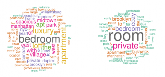
The name variable will be used in order to analyse how hosts promote their listing, as it is one of the things potential guests see at first. More specifically, in the following it will be analysed, what words are used most frequently in the title and how these words differ between cheap and expensive listings. Therefore, the titles of the cheapest 15% and the most expensive 10% of the listings are used. The figure below shows the wordcloud (containing the most frequently used words) for cheap and expensive listings.

# remove unwanted characters from the titles
pattern = paste("/", "@", "/|", "+", "!", "w", "-", "1", "2", "3", "4", "a", "in", ",", sep=" | ")
listings$name = gsub(pattern, " ", listings$name)

#creating a dataframe for the expensive listings (listings after the 90th quantile or the most expensive, 10% of the listings)
quant_90 = as.numeric(quantile(listings$price, 0.9), na.rm = TRUE)
title_exp = listings[listings$price > quant_90, "name"]
word_counts_exp = data.frame(table(unlist(strsplit(tolower(title_exp), " "))))

#creating a dataframe for the affordable listings (listings of the 15th quantile or the cheapest, 15% of the listings)
quant_15 = as.numeric(quantile(listings$price, 0.15), na.rm = TRUE)
title_cheap = listings[listings$price < quant_15, "name"]
word_counts_cheap = data.frame(table(unlist(strsplit(tolower(title_cheap), " "))))

# Fig. 1
# creating two wordcloud visualisations
par(mfrow=c(1,2))

wordcloud(words = word_counts_exp$Var1, freq = word_counts_exp$Freq, min.freq = 5,
          max.words = 82, random.order = F, colors = brewer.pal(8, "Dark2"))

wordcloud(words = word_counts_cheap$Var1, freq = word_counts_cheap$Freq, min.freq = 5,
          max.words = 60, random.order = F, colors = brewer.pal(8, "Dark2"))

Fig. 1: Wordcloud visualisations of the most frequently used words in titles of expensive (left) and the cheap (right) Airbnb listings.

Most Airbnb hosts seem to promote the property type of their accommodation, like loft or apartment, as well as the location it is situated in, like Manhattan.

Moreover, it stands out that the expensive listings contain words like luxury, beautiful and modern in their titles, while cheaper listings rather use euphemisms like cozy, spacious and comfy.

Based on this knowledge, we can now track if a listing's title includes one of the most frequently used words for one or the other price category.

#creating two lists with the most frequent words in the titles for expensive and cheap listings
words_cheap = c("spacious", "charming", "cozy", "columbia", "convenient", "affordable")

words_exp = c("luxury", "amazing", "garden", "gorgeous", "best", 
              "stunning", "terrace", "luxurious", "times square")

#creating a function to count the number of words of interest (words_a) in the whole title (words_b)
count_word_matches = function(words_a, words_b){
  if(sapply(strsplit(words_a, " "), length) == 0){
    return(0)
  }
  else{
    return(sum(sapply(strsplit(tolower(words_a), " "), function(x) x %in% words_b)))
  }
}

#creating two variables with the function applied
num_words_cheap = sapply(listings$name, 
                         function(x) count_word_matches(as.character(x), words_cheap))

num_words_exp = sapply(listings$name, 
                       function(x) count_word_matches(as.character(x), words_exp))


#adding the two new variables to the listings dataframe
listings = cbind(listings, num_words_cheap, num_words_exp)

Choropleth map

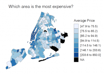
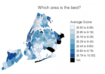
Next, the price differences between different areas of New York will be analysed. Therefore, the zipcodes will be used to group areas together and calculate their mean prices. In a second step, it will be analysed whether the price and the location rating score are correlated, as the latter is a continuous variable and could therefore be used easily as a predictor for the price, while the zipcode is a categorical variable, consisting of 206 levels, which would result in 206 (binary) dummy variables and make prediction difficult.

The code below calculates the average price per zipcode and plots the result on a map of New York. Analogous, the plot for the average location score per region is created.

Fig. 2: Visualisation of New York areas with a choropleth map, categorised by the average price

# Fig. 2
zipcode_prices <- listings %>% 
  group_by(zipcode = zipcode) %>% 
  summarise(avg_loc_review = mean(price, na.rm = TRUE))

colnames(zipcode_prices) <- c("region","value")

zipcode_prices$region <- as.character(zipcode_prices$region)

nyc_fips = c(36005, 36047, 36061, 36081, 36085)

g_locations_price <- zip_choropleth(zipcode_prices, 
                                    county_zoom = nyc_fips, 
                                    title = "Average Prices by Region", 
                                    legend = "Average Price") + 
  ggtitle("Which area is the most expensive?") +
  theme(legend.text = element_text(size=7),
        legend.key.size = unit(0.4, "cm"), 
        legend.title = element_text(size=8), 
        plot.title = element_text(size=10, hjust = 1.5))

Fig. 2: Visualisation of New York areas with a choropleth map, categorised by the average rating score

# Fig. 3
zipcode_scores <- listings %>% 
  group_by(zipcode = zipcode) %>% 
  summarise(avg_loc_review = mean(review_scores_location, na.rm = TRUE))

colnames(zipcode_scores) <- c("region","value")

zipcode_scores$region <- as.character(zipcode_scores$region)

nyc_fips = c(36005, 36047, 36061, 36081, 36085)

g_locations_score <- zip_choropleth(zipcode_scores,
                              county_zoom = nyc_fips,
                              title = "Location Review Scores by Region",
                              legend = "Average Score") + 
  ggtitle("Which area is the best?") + 
  theme(legend.text = element_text(size=7), 
        legend.title = element_text(size=8),
        legend.key.size = unit(0.4, "cm"), 
        plot.title = element_text(size=10, hjust = 1.5))

#grid function puts two plots in a row, if necessary
plot_grid(g_locations_price, g_locations_score, nrow=1)

From the plots, one can infer that a higher location score indicates a higher price. The correlation coefficient is calculated below:

zipcode_scores_prices = zipcode_scores %>% 
  inner_join(zipcode_prices, by = "region")

zipcode_scores_prices = zipcode_scores_prices[complete.cases(zipcode_scores_prices), ]
cor(zipcode_scores_prices$value.x, log(zipcode_scores_prices$value.y))

## Output:
## [1] 0.3830552

And with almost 0.4 one can conclude, that there is a positive correlation between the location score and the price of a listing. Note that the correlation coefficient is calculated based on the logarithm of the price, as the price is highly skewed towards very high prices.

Scatter plot and Boxplots

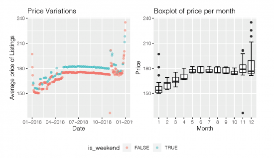
Next, the calendar data will be analysed. The focus here is wheather there are seasonal patterns in the price which should be included in the machine learning model for price prediction.

calendar2017 <- read.csv("calendar2017.csv")
calendar2018 <- read.csv("calendar.csv")
calendar <- rbind(calendar2017, calendar2018)
calendar = calendar[year(calendar$date) == 2018, ]
rm(list = c("calendar2017", "calendar2018"))

### Fig. 4
### Seasonal analysis #####

calendar$price <- as.numeric(gsub(",", "", substring(calendar$price, 2)))

seasonal_df <- calendar %>% 
  group_by(date = date) %>% 
  summarise(avg_price = mean(price, na.rm = TRUE)) %>% 
  mutate(year = year(date))

seasonal_df$date = as.Date(seasonal_df$date)

# make a feature that indicates whether a day is a friday or a saturday
# These are potentially the days where the prices for a night are the highest

seasonal_df$dayofweek = wday(seasonal_df$date)
is_weekend = seasonal_df$dayofweek %in% c(6, 7)
seasonal_df$is_weekend = factor(is_weekend)

# make a scatter plot of the daily average prices
g_scatter = ggplot(seasonal_df, aes(date, avg_price)) + 
  geom_point(aes(color=is_weekend), alpha=0.5) +
  ggtitle("Price Variations") +
  labs(x = "Date", y = "Average price of Listings") + 
  scale_x_date(date_labels = "%m-%Y")

# make a boxplot of the price across the different months

g_box = ggplot(seasonal_df, aes(as.factor(month(date)), avg_price)) + 
  geom_boxplot() + 
  stat_boxplot(geom = "errorbar", width = 0.5) + 
  ggtitle("Boxplot of price per month") + 
  labs(x = "Month", y = "Price")

# make a grid of both plots being in a row

prow = plot_grid(g_scatter + theme(legend.position = "none"),  
                 g_box + theme(legend.position = "none"),
                 nrow=1)

# create a legend for the scatter plot and put it in a new row of the grid

legend = get_legend(g_scatter + theme(legend.position = "bottom"))
plot_grid(prow, legend, ncol=1, rel_heights = c(1,.2))

Fig. 4: Correlation between the price and the day of the week (left, scatter plot) as well as the month (right, boxplots)

What immediately stands out is the affect of weekends on the price. Renting an appartment on Airbnb on a Friday or Saturday seems to be more expensive compared to other weekdays. However, this effect is a little bit exaggerated in this plot, as it is not scaled between zero and the upper bound. In fact, the relative difference in price between weekdays and non weekdays, is only about 3%.

a = mean(seasonal_df[(seasonal_df$is_weekend == T), ]$avg_price)
b = mean(seasonal_df[(seasonal_df$is_weekend == F), ]$avg_price)
abs(a-b)/b

## Output:
## [1] 0.03695569

Another thing that strikes attention is the monthly pattern in the price. Especially the difference between late December and the first months of a year seems to be big. Looking at the boxplot of the price per month there is a clear monthly seasonality visible.

Feature Engineering

In order to train a model that makes predictions for the price of a specific Airbnb accommodation, meaningful features have to be created which the supervised learning model can take as input to derieve patterns in the data that determine the prices of the very many accommodations in the data set.

The exploratory data analysis was very helpful for this, as it has revealed many determinants for the price already. For example, seasonality plays an important role for the price, hence need to be included in the model.

First of all, the two tables need to be merged into one data frme, which contains all the information that is needed. The `calendar` data frame contains over 16mio. observations, hence is computationally very heavy. Therefore, the table will be reduced by sampling randomly `r sample_length` observations from it (without replacement).

Fig.5

listings = listings[, -which(colnames(listings) %in% c("price", "zipcode"))]
listings = listings[complete.cases(listings), ]
colnames(listings)[which(colnames(listings) == "neighbourhood_group_cleansed")] = "neighbourhood"
calendar = calendar[, -which(colnames(calendar) %in% c("available"))]
calendar = calendar[complete.cases(calendar), ]
sample_length = 100000

df_panel = calendar %>% inner_join(listings, by = c("listing_id" = "id"))
df_panel = df_panel[complete.cases(df_panel), ]
samples = sample(c(1:dim(df_panel)[1]), sample_length)
df_panel = df_panel[samples, ]

#visualising the dataframe
text_tbl <- data.frame(
  c1 = colnames(df_panel)[1:11], 
  c2 = c(colnames(df_panel)[c(12:21)], "")
)

kable(text_tbl, col.names = NULL) %>%
  kable_styling() %>%
  column_spec(1) %>%
  column_spec(2)

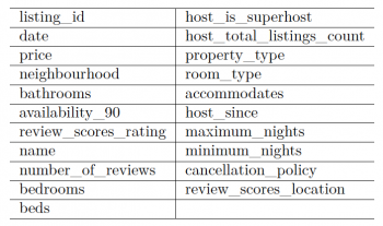
The resulting data frame can be seen on Figure 5. A lot of the variables in the data are categorical (nominal). Many machine learning algorithms cannot operate on nominal data directly. They require all input variables and output variables to be numeric.

To achieve that, the nominal variables have to be one-hot encoded. This means that each distinct value of the variable is transformed into a new binary variable (source).

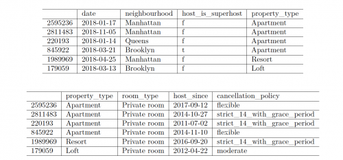
First, all categorical variables will be determined.

Fig. 6

#Fig. 6
cat_vars = names(which(sapply(df_panel, class) == "factor"))
df_cat = df_panel[, which(colnames(df_panel) %in% cat_vars)]
head(df_cat[, c(1:4)]) %>% 
  kable() %>% 
  kable_styling()

cat_vars = names(which(sapply(df_panel, class) == "factor"))
df_cat = df_panel[, which(colnames(df_panel) %in% cat_vars)]
head(df_cat[, c(4:dim(df_cat)[2])]) %>% 
  kable() %>% 
  kable_styling()

Not for all these variables it makes sense to create a new binary variable for each of the distinct values, as they just contain to many different values or even contain only values that are unique, like the names variable. These variables need to be transformed in a more logical way. For example the host_since variable. This can be transformed into an integer variable by calculating the difference in days between the date the host joined Airbnb and the date of the listing being offered.

df_panel$host_since = abs(as.integer(difftime(df_panel$date, df_panel$host_since)))

cat_vars = cat_vars[cat_vars %in% "host_since" == FALSE]

Moreover, the date variable would not provide a lot of information if each date would be transformed into a new binary variable. However, as has been shown in the exploratory data analysis, there are a lot of seasonal influences on the price that can be captured by the date. Therefore, the date variable will be transformed into two new columns. One column that specifies the month an accommodation is being offered and another column specifing the day of the week in which the accommodation can be rented. Monthly and daily seasonalities (especially weekends) seemed to be the most influencial.

df_panel = df_panel %>% 
  mutate("month_of_year" = month(date)) %>% 
  mutate("dayofweek" = wday(date))

cat_vars = cat_vars[cat_vars %in% "date" == FALSE] 
cat_vars = c(cat_vars, "month_of_year", "dayofweek")

Lastly, the name variable does not contain any information as well without further processing. As has been shown earlier, there are certain words, which are used to promote expensive as well as rather cheap accommodations. The words that have been identified there will be used now. For each title of an Airbnb listing, the number of words that are used from the set of words used to promote expensive flats is determined (as well as the number of words used to promote cheaper accommodations). These features will be saved as num_words_exp and num_words_cheap respectively.

words_cheap = c("spacious", "charming", "cozy", "columbia", "convenient", "affordable")
words_exp = c("luxury", "amazing", "garden", "gorgeous", "best", 
              "stunning", "terrace", "luxurious", "times square")
# function that returns the number of words_b that appear in words_a
count_word_matches = function(words_a, words_b){
  if(sapply(strsplit(words_a, " "), length) == 0){
    return(0)
  }
  else{
    return(sum(sapply(strsplit(tolower(words_a), " "), function(x) x %in% words_b)))
  }
}
num_words_cheap = sapply(df_panel$name, 
                         function(x) count_word_matches(as.character(x), words_cheap))
num_words_exp = sapply(df_panel$name, 
                         function(x) count_word_matches(as.character(x), words_exp))
df_panel = cbind(df_panel, num_words_cheap, num_words_exp)

cat_vars = cat_vars[cat_vars %in% "name" == FALSE]

The other categorical variables can now be transformed using one-hot encoding. After that, all categorical variables will be removed from the data frame.

dmy = dummyVars(" ~ .", data = df_panel[, cat_vars])
dmy = predict(dmy, newdata = df_panel[,cat_vars])
df_panel = cbind(df_panel, dmy)

df_panel = df_panel[, -which(colnames(df_panel) %in% c(cat_vars, "name", "date", "host_since"))]

# delete those entries where the price is zero
df_panel = df_panel[df_panel$price != 0, ]

Model training

To predict the price (a numeric variable) a regression model has to be used. There are, after all the feature engineering and one-hot encoding, 66 explanatory variables in the data set and probably a lot of interactions between these variables. For example, a big apartment in a suburb of New York, far away from the city center might be nothing special and therefore not extremely expensive. If the same sized flat, however, is located in the middle of Manhatten, the price would be huge.

Therefore, a Random Forest will be used in order to determine the price of an accommodation. A Random Forest is an ensemble learning model. It consists of many weak regression models, namely decision trees which are allowed only to make a small number of splits. In a decision tree, we can split branches by one variable first then split again by another variable. This is essentially creating interactions and thus is a good model class for the problem at hand.

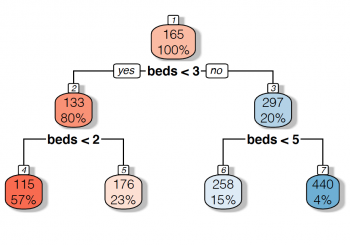
Moreover, having so many variables can cause a single model to overfit, hence leading to bad prediction results on observations that have not been used for training the model. A Random Forest however uses a lot of small decision trees, where each of them is not able to overfit as it cannot grow large enough to capture all the patterns of the target and additionally uses only a small (random) subset of the whole feature space. The plot on Figure 7 shows an example of a small decision tree for price prediction, where the large number in each of the nodes specifies the predicted price.

Fig. 7

#Fig. 7
tree = rpart(price~beds, data = df_panel)
rpart.plot(tree, box.palette = "RdBu", shadow.col = "gray", nn=T)

The following code snipped first generates a matrix X that contains all explanatory variables and second a vector _y_ containing all the prices for the respective listings. After that, the matrix _X_ and the vector y are splitted into a train and a test set, where the train set is used to build the Random Forest regression model and the test set to validate its predictive power.

X = df_panel[, -which(colnames(df_panel) %in% c("price", "listing_id"))]
y = log(df_panel$price)
train = sample(1:dim(X)[1], 0.7*dim(X)[1], replace = F)
X_train = X[train, ]
y_train = y[train]
rfr = randomForest(X_train, y_train, maxnodes=15, ntree=1000, importance=TRUE)
y_pred = exp(predict(rfr, X[-train,]))
y_test = exp(y[-train])
mape = mean(abs(y_test - y_pred) / y_test) #calculating the mean absolute percentage error
print(paste0("The MAPE of the Model is ", round(mape*100,2), " percent"))

## Output:
## [1] "The MAPE of the Model is 31.72 percent"

Result and Conclusion

This short report attemted to predict the price of an overnight stay in an Airbnb accommodation based on various features. These features have to a large extend been generated based on insights gained through exploratory data analysis. The overarching aim was here to explain determinants of the price of an Airbnb accommodation. The prediction is based on a Random Forest, which results in a mean absolute percentage error of around 30% on the test set. The interpretation for this measure is, that on average the predicted price deviates by 30% from the actual one, which is quite high. Therefore, important influences on the variablity of the price have not been captured, i.e. important features have not been identified throughout this report. One of these neglected features could be for example information about holidays. For instance, the average price for an accomodation rose steadily a few days before Christmas and New Year, something that should be captured by the model.

Moreover, due to computational limitations, the hyperparameters of the Random Forest have not been tuned and not all observations could be used to train and validate the model, leading to results worse than what could have actually been achieved.

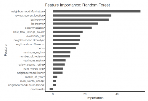
Nonetheless, to a large extend the model developed during this report already captures the patterns of the variation in price across different listings on different days quite well. The following list contains the 15 most important variables to explain the price:

Fig. 8

#Fig. 8
# make dataframe from importance() output
feat_imp_df <- importance(rfr) %>% 
  data.frame() %>% 
  mutate(feature = row.names(.))
feat_imp_df = feat_imp_df[c(1:20), ]
# plot dataframe
ggplot(feat_imp_df, aes(x = reorder(feature, X.IncMSE),
                        y = X.IncMSE, width=.5)) +
  geom_bar(stat='identity') +
  coord_flip() +
  theme_classic() +
  labs(
    x     = "Feature",
    y     = "Importance",
    title = "Feature Importance: Random Forest"
    )

---

The author of this entry is Laurin Luttmann.