Introduction to statistical figures
Contents
Basic forms of data visualisation
This section introduces you to the most relevant forms of data visualisation. For R examples, please check the section below.
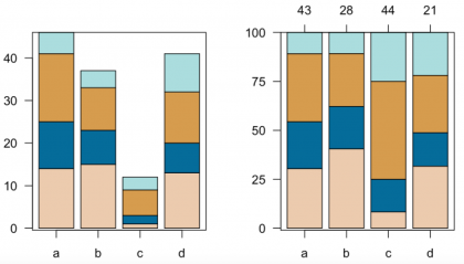
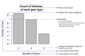
The easiest way to represent count information are basically barplots. They are a bit over simplistic if they contain only one level of information such as three groups and their abundance, and can be more advanced if they contain two levels of information such as in stacked barplots. These can be shown as either absolute numbers or proportions, which may make a dramatic difference for the analysis or interpretation.
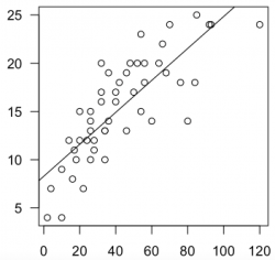
Correlation plots ('xyplots') are the next staple in statistical graphics and most often the graphical representation of a correlation. Further, often also a regression is implemented to show effect strengths and variance. Fitting a regression line is often the most important visual aid to showcase the trend. Through point size or color can another information level be added, making this a really powerful tool, where one needs to keep a keen eye on the relation between correlation and causality. Such plots may also serve to show fluctuations in data over time, showing trends within data as well as harmonic patterns.
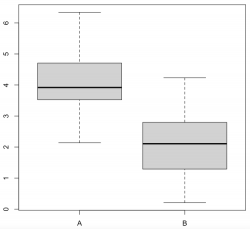
Boxplots are the last in what I would call the trinity of statistical figures. Showing the variance of continuous data across different factor levels is what these plots are made of. While histograms reveal more details and information, boxplots are a solid graphical representation of the Analysis of Variance. A rule of thumb is that if one box is higher or lower than the median (the black line) of the other box, the difference may be signifiant.
A histogram is a graphical display of data using bars (also called buckets or bins) of different height, where each bar groups numbers into ranges. They can help reveal a lot of useful information about numerical data with a single explanatory variable. Histograms are used for getting a sense about the distribution of data, its median, and skewness.
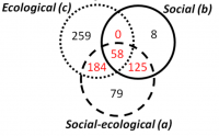
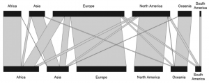
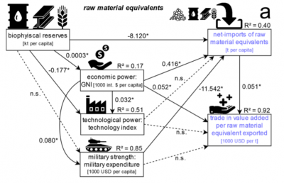
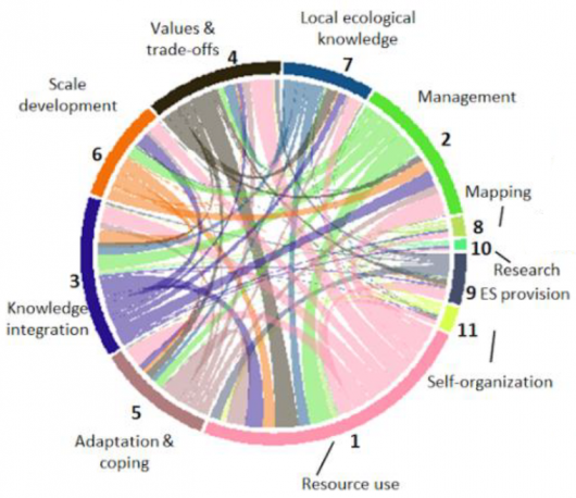
Simple pie charts are not really ideal, as they camouflage the real proportions of the data they show. Venn diagrams are a simple way to compare 2-4 groups and their overlaps, allowing for multiple hits. Larger co-connections can either be represented by a bipartite plot, if the levels are within two groups, or, if multiple interconnections exist, then a structural equation model representation is valuable for more deductive approaches, while rather inductive approaches can be shown by circular network plots (aka Chord Diagram).
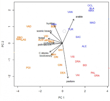
Multivariate data can be principally shown by three ways of graphical representation: ordination plots, cluster diagrams or network plots. Ordination plots may encapsulate such diverse approaches as decorana plots, principal component analysis plots, or results from a non-metric dimensional scaling. Typically, the first two most important axis are shown, and additional information can be added post hoc. While these plots show continuous patterns, cluster dendrogramms show the grouping of data. These plots are often helpful to show hierarchical structures in data. Network plots show diverse interactions between different parts of the data. While these can have underlying statistical analysis embedded, such network plots are often more graphical representations than statistical tests.
Descriptive Infographics can be a fantastic way to summarise general information. A lot of information can be packed in one figure, basically all single variable information that is either proportional or absolute can be presented like this. It can be tricky if the number of categories is very high, which is when a miscellaneous category could be added to a part of an infographic. Infographics are a fine art, since the balance of information and aesthetics demands a high level of experience, a clear understanding of the data, and knowledge in the deeper design of graphical representation.
Of course, there is more. While the figures introduced above represent a vast share of the visual representations of data that you will encounter, there are different forms that have not yet been touched. We have found the website "From data to Viz" to be extremely helpful when choosing appropriate data visualisation. You can select the type of data you have (numeric, categoric, or both), and click through the exemplified figures. There is also R code examples.
How to visualize data in R
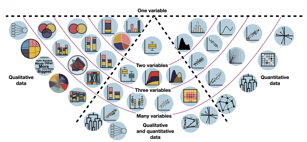
The following overview includes all forms of data visualisation that we consider important.
Based on your data, have a look which forms of visualisation might be relevant for you. Just hover over the individual visualisation type and it will show you its name. It will also show you a quick example which this kind of visualisation might be helpful for. By clicking, you will be redirected to a dedicated entry with exemplary R code.
Tip: If you are unsure whether you have qualitative or quantitative data, have a look at the entry on Data formats. Keep in mind: categorical (qualitative) data that is counted in order to visualise each category's occurrence, is not quantitative (= numeric) data. It's still qualitative data that is just transformed into count data. So the visualisations on the left do indeed display some kind of quantitative information, but the underlying data was always qualitative.
The following section provides some examples and R code for simple forms of data visualisation. For more info on data formats, please refer to Data formats.
Barplots
– in Barplots, Histograms and Boxplots
Boxplot
– in Barplots, Histograms and Boxplots
Histogram
– in Barplots, Histograms and Boxplots
Scatter Plot
– in Correlation plots
Line chart
– in Correlation plots
ggplot
– in Correlation plots
Venn diagrams
– in Venn diagrams
Pie chart
– in Pie Charts
Other statistical figures
As mentioned above, we have found the website "From data to Viz" to be extremely helpful when choosing appropriate data visualisation. You can select the type of data you have (numeric, categoric, or both), and click through the exemplified figures. There is also R code examples.
Further visualisation examples on this Wiki:
- Clustering methods
- Ordination and Network Analysis
- Chord Diagram
- Kernel density plot
Graphical etiquette – a rough guide how to make scientific quantitative figures
There is an almost uncountable amount of scientific figures out there. While diversity is great, it can often be overwhelming to consider which graphics to do with data, and which other types of figures can be beneficial. In addition, there are some general norms and conventions to consider when making graphics. Let us start with these. While these are mere suggestions, and reflect my own style and experience, they may serve as a reflection basis for others.
1) Only show data in a figure that contains enough information to justify a figure
Many barplots I have seen contain 2 values. Could these not be fit into a sub-sentence? A graphic is to this end downright trivial, and wastes a lot of space. The same is also true for a piechart, but even worse, because it can look like a Pacman, and pie-charts are just generally misleading. Hence consider how many values you want to show, and if these really justify the journal space.
2) One should not show plots that violate the statistics
A common example are barplots. There can be good reasons to show barplots with error bars, however the majority of data is better represented by a boxplot. Boxplots show more values, and are sensible for data that contains a range of integers. A typical borderline case is the Likert Scale, which is often shown in boxplots. While this is not entirely wrong, it is a bit strange, as the scale contains five values, and a boxplot is constructed of five parts at least. Another example is the standard fitted loess line in a ggplot. If you show non-linear statistics, there should be a reason for it. Some of these trends show nothing at all, and follow no assumption beside adding some graphical interest. Scientific figures are however not only about aesthetics, but also about soundness and validity.
3) Avoid empty spaces in plots. After all, your graphics are no Zen garden
Speaking of aesthetics, your plots should be balanced, and should not contain open spaces. Try to set the x and y axes in a way that empty space is avoided. Such space could be ideal for a legend, or maybe some other additional information. Often people use weird short names in the legend, and then explain them in the figure caption. This should be avoided at all costs. Try to create legends that are self-explanatory. Make sure that the density of the information that is being shown is balanced, at least as long as the data and analysis allows for this. If figures contain much open space you can still definitely try to make them smaller, and maybe even combine several of these in a panel plot. In certain graphics such as clearcut correlations empty space is hard to avoid. This is a good indicator that maybe this figure is not needed at all, but instead can be replaced by some relevant values (e.g. p-value, R2 ) in the text.
4) Use diverse, but also non-confusing colours
I am colourblind, so I am in the privileged position to judge on the diversity of colours in a plot. Actually, no test ever picked up any colour blindness, but I definitely have some problem there. Hence I would say that colours should be diverse, and ideally brightness and hue allow also to differentiate groups. Figures become problematic if there are too many colours, and I define this threshold for me at around 8. In addition, consider using colours that have proven their value when combined. I can endorse weandersonpalette as a really cool package that gives you a pleasing combination of colours.
5) Label orientation goes a long way
Most label orientations in most plots are wrong. Try to bring your labels -if space permit- into a horizontal orientation. quite often tables are too densely packed on the x-axis then, yet you could also consider making them in a 45 ° fashion. As much as a 90 ° label orientation can offer a little stretch for the neck, it is also a one-sided exercise. Hence consider flipping the labels whenever possible.
6) Compose the figure right to its intended size
One of the most common mistakes in the creation of figures is the proportion of different parts of the figure. Often the axes labels are really small, but the heading is massive. Ideally when designing a figure, one should consider to size with which this figure should be printed. If you know that a figure is only 6x6 centimetres, you need to make the labels sufficiently large and sparse to be readable, and orderly. A larger figure has different proportions. Hence design your figures in the right composition interns of the different text sizes.
7) Use one font only
Ok, font types are like borderline religion, but still I guess we can all agree that one should only use one font in a figure. If you want to make a typesetter cry you may use one font with serifs and another one without serifs, but otherwise do not do that. It can make sense to use a narrow font (iei. Arial narrow) if you do not have enough space in your figure.
8) Occam's razor applies to scientific figures, too
A good figure is balanced, and ideally contains as much information as possible, but not more. You can however also decide to make figures that contain more information, and are borderline like mandalas. This is really cool if you have complex information to show for, and maybe the result basically says that it's complex. Other figures may be graspable in a split second, which is very cool if you want people to understand something quickly. In between is the Occam's razor sweet spot, where you need a few seconds with the figure, but then you kind of got it. To this send, let it be known that this sweet spot is different for different people.
The author of this entry is Henrik von Wehrden.
