Likert Scale
In short: Likert Scales are categorical ordinal scales that are used in surveys to measure attitude. They are widely used in Social Sciences, but also in employee surveys when asking about satisfaction in the job or in customer surveys where products/services can be rated.
Contents
Background
The name of the scale comes from the American psychologist Rensis Likert. In 1932, Likert developed a 7-point agreement scale out of interest in measuring people’s opinions and attitudes. His initial scale is very similar to the ones used today.
What do Likert Scales look like?
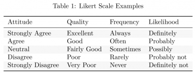
The most common Likert Scale asks for attitude on 5 different levels: Strongly Agree, Agree, Neutral/Undecided, Disagree, and Strongly Disagree. Other options include 3 or 7 answer options. Odd numbers are commonly used to include a neutral or undecided option in the middle. If no such neutral option is added, we call the scale a forced-choice method, because respondents are forced to decide if they are leaning more against the agree or disagree side of the scale. Sometimes, opt-out responses are also used, such as “I don’t know” or “Not applicable”. Those are then placed outside the scale. Apart from attitude, Likert scales can also be used to measure other variations such as quality, frequency or likelihood to give some examples. In online surveys, a variant with a kind of slider has been used more and more recently: In this variant, respondents can indicate their answer on a scale from zero (minimum) to 100 (maximum).
install.packages("dplyr")
install.packages("kableExtra")
install.packages("ggplot2")
library(kableExtra)
library(dplyr)
library(ggplot2)

df <- data.frame(
  Attitude = c("Strongly Agree", "Agree", "Neutral", "Disagree", "Strongly Disagree"),
  Quality = c("Excellent", "Good","Fairly Good", "Poor", "Very Poor"),
  Frequency = c("Always", "Often", "Sometimes", "Rarely", "Never"),
  Likelihood = c("Definitely", "Probably", "Possibly", "Probably not", "Definitely not"))

kbl(df, booktabs = T, caption = "Likert Scale Examples") %>%
  kable_styling(latex_options = c("striped", "hold_position"),
                full_width = F)
How to analyze Likert Scales & Visualization in R
Even though one may find that analyzing Likert Scales looks fairly easy and straight forward, there is a huge debate on how to analyze these scales correctly. The biggest point of conflict in the discussion is whether the scale can be considered ordinal or interval. While Likert Scales technically are ordinal data, because there clearly is a grading: "Strongly Agree" is graded higher than "Agree", strictly speaking, the assumption of equal distance between categories is not valid. That is, the distance between “Agree” and “Neutral” theoretically is not the same as the distance between “Neutral” and “Not Agree”. That is why, we would strictly not consider Likert Scales as interval scaled, where each distance should be equal.
However, in some areas, it is accepted to apply parametric statistics for Likert Scales, such as calculating a mean, doing an ANOVA or t-test, which means treating them as an interval. Cases in which Likert Scales can be treated as intervals are if there are a high number of response options per question, when response options are assumed to be equally spaced, or when respondents mark their answer on a line so that the precise location of the mark can be measured. Making a decision about which method to apply, one should look at the literature of its discipline, reflect the assumption for each method and apply the method which is widely accepted in its field.
1. Coding the Responses
Statements in a survey are often differently framed. While some are framed positively, for instance, the participant may be asked for its attitude to the statement “I am satisfied with what I learned this semester”, others are framed negatively, like “I am not satisfied with the course offer this semester”. The different framing is used to check for respondents who do not read the question and just click the same answer every time. In a statistical analysis, it may be useful to recode the responses, so that each response is going in the same logical direction when 0 is "Strongly Disagree", 1 is "Disagree", and so on. Let’s see how that works with an example dataset I will construct here.
#construct a random dataset
set.seed(5) # random number will generate from 5
satisfaction_learning <- floor(runif(100, min=0, max=5)) #construct 100 random responses of range 0 to 100
dissatisfaction_semester <- floor(runif(100, min=0, max=5))
sex <- floor(runif(100, min = 0, max = 2))

# We want 100 responses with satisfaction_learning being coded 0 = Strongly Disagree, 1 = Disagree...
# We recode dissatisfaction_semester to satisfaction_semester by making the opposite: 4 = Strongly Disagree,
#3 = Disagree, etc.

df <- data.frame(id = 1:100,
                 sex = case_when(sex == 0 ~ "man",
                                 sex == 1 ~ "woman"),
                 satisfaction_learning = case_when(satisfaction_learning == 0 ~ "Strongly Disagree",
                                                   satisfaction_learning == 1 ~ "Disagree",
                                                   satisfaction_learning == 2 ~ "Neutral",
                                                   satisfaction_learning == 3 ~ "Agree",
                                                   satisfaction_learning == 4 ~ "Strongly Agree"),
                 satisfaction_semester = case_when(dissatisfaction_semester == 4 ~ "Strongly Disagree",
                                                   dissatisfaction_semester== 3 ~ "Disagree",
                                                   dissatisfaction_semester == 2 ~ "Neutral",
                                                   dissatisfaction_semester == 1 ~ "Agree",
                                                   dissatisfaction_semester == 0 ~ "Strongly Agree"))

# Create a function to calculate the mode of the given responses
getmode <- function(v) {
  uniqv <- unique(v)
  uniqv[which.max(tabulate(match(v, uniqv)))]
}
print(mode_satis_learning <- getmode(df$satisfaction_learning))
print(mode_satis_semester <- getmode(df$satisfaction_semester))
2. Descriptive Statistics
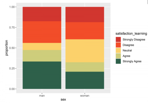
To analyze Likert Plots, one can have a look at the results in a descriptive way at first. That means, looking at the mode (which is the most frequent response) and plotting the percentages of people who disagree, agree etc., in a stacked barplot, a graph or one bar for each response.
In our example data, "Strongly Agree" is the mode for the statement of being satisfied with what one learned this semester and "Agree" is the most frequent answer for the satisfaction of the course offered this semester. Let’s plot the learning satisfaction ratings of all the participants in one stacked barplot with percentages per gender.
# We need the label Agreement for our colors later
df$satisfaction_learning <- ordered(df$satisfaction_learning,
                                    levels = c("Strongly Disagree", "Disagree",
                                               "Neutral", "Agree", "Strongly Agree"))

# We have to put the labels in order
df$satisfaction_learning <- ordered(df$satisfaction_learning,
levels = c("Strongly Disagree", "Disagree", "Neutral",

# Create a unique color palette (I like to use colors from Wes Anderson movies)
col_pal_satisf <- tibble(
  agreement = c("Strongly Disagree", "Disagree", "Neutral", "Agree", "Strongly Agree"),
  colors = c(c("#D1362F", "#F24D29", "#FCD16B", "#CECD7B", "#2E604A")))
sum_satisfaction_learning <- df %>%
  group_by(sex, satisfaction_learning) %>%
  summarise(n = n()) %>%
  group_by(sex) %>%
  mutate(proportion = n/sum(n))
sum_satisfaction_learning %>%
  ggplot(aes(sex, proportion, fill = satisfaction_learning)) +
  geom_col() +
  scale_fill_manual(values = setNames(as.character(col_pal_satisf$colors), col_pal_satisf$agreement))
3. Inference Statistics
The last step now really depends if we would treat the scale as ordinal or interval. Here are some analysis options for when treating the scale as ordinal or reducing it to a binary variable. If it is treated as an interval, any parametric test (ANOVA, Linear Regression, etc.) can be computed.
If treating scale as ordinal
- Ordinal Regression
Here, the dependent variable is ordinal in the regression. The ordinal package in R provides a powerful and flexible framework for ordinal regression. It can handle a wide variety of experimental designs, including those with paired or repeated observations. Look here for more on Ordinal Regressions in R.
- Tests for ordinal
Tests for ordinal data are arranged in a contingency table form. These include the linear-by-linear test, which is a test of association between two ordinal variables, or the Cochran-Armitage test. This is a test of association between an ordinal variable and a nominal variable. One has to consider though, that these tests are limited to data arranged in a two-dimensional table and they require spacing between ordinal categories. More information can be found here.
- Permutation tests
One can use the coin package in R to run permutation tests with ordinal dependent variables. It can handle models analogous to a one-way analysis of variance with stratification blocks, including paired or repeated observations. For more information on these tests visit this link.
If reducing scale to a binary variable
Sometimes, it is acceptable to reduce the responses of a Likert Scale to only two responses: summing up for instance “Strongly Agree” and “Agree” to one category, and “Strongly Disagree” and “Disagree” to another category and dropping the neutral response. In this case, lots of information will get lost, but if there is a strong argumentation for this step in the research, it is valid to do so. In this case, one can do a Logistic Regression if the dependent variable is the Likert Scale or just add a dummy variable in a Linear Regression if the independent variable is ordinal.
The author of this entry is Nora Pauelsen.

