Causality
Note: This entry focuses on Causality in science and statistics. For a brief summary of the relation between Causality and Correlations, please refer to the entry on Causality and correlation.
Contents
Introduction
Causality. Where to start, how to end?
Causality is one of the most misused and misunderstood concepts in statistics. All the while it is at the heart of the fact that all statistics are normative. While many things can be causally linked, other things are not causally linked. The problem is that we dearly want certain things to be causally linked, while we want other things not to be causally linked. This confusion has many roots, and spans across such untameable arenas such as faith, psychology, culture, social constructs and so on. Causality can be everything that is good about statistics, and it can be equally everything that is wrong about statistics. To put it in other words, it can be everything that is great about us humans, but it can be equally the root cause of everything that is wrong with us.
What is attractive about causality? People search for explanations, and this constant search is probably one of the building blocks of our civilisation. Humans look for reasons to explain phenomena and patterns, often with the goal of prediction. If I understood a causal relation, I may be able to know more about the future, cashing in on being either prepared for this future, or at least being able to react properly.
The problem with causality is that different branches of science as well as different streams of philosophy have different explanations of causality, and there exists an exciting diversity of theories about causality. Let us approach the topic systematically.
The high and low road of causality
Let's take the first extreme case, building on the theory that storks bring the babies. Obviously this is not true. Creating a causal link between these two is obviously a mistake. Now lets take the other extreme case, you fall down a flight of stairs, and in the fall break your leg. There is obviously some form of causal link between these two actions, that is falling down the stairs caused you to break your leg. However, this already demands a certain level of abstraction, including the acceptance that it was you who did fall down the stairs, you twisting your leg or hitting a stair with enough force, you not being too weak to withstand the impact etc. There is, hence, a very detailed chain of events happening between you starting to lose your balance, and you breaking your leg. Our mind simplifies this into “because I fell down the stairs, I broke my leg”. Obviously, we do not blame the person who built the stairs, and we do not blame our parents for bringing us into this world, where we then broke our leg. These things are not causally linked.
But, imagine now that the construction worker did not construct the stairs the proper way, and that one stair is slightly higher than the other stairs. We now claim that it is the fault of the construction worker. However, how much higher does this one stair need to be so that we blame not ourselves, but the construction worker? Do you get the point?
Causality is a construction that is happening in our mind. We create an abstract view of the world, and in this abstract view we come of with a version of reality that is simplified enough to explain for instance future events, but it is not too simple, since this would not allow us to explain anything specific or any smaller groups of events.
Causality is hence an abstraction that follows the Occam's Razor, I propose. And since we all have our own version of Occam's Razor in our head, we often disagree when it comes to causality. I think this is merely related to the fact that everything dissolves under analysis. If we analyse any link between two events then the causal link can also be dissolved, or can become irrelevant. For this reason, a longer discussion was needed to clarify that, ultimately, causality is a choice.
Take the example of medical studies where most studies build on a correlative design, testing how, for instance, taking Ibuprofen may help against the common cold. If I have a headache, and I take Ibuprofen, in most cases it may help me. But do I understand how it helps me? I may understand some parts of it, but I do not really understand it on a cellular level. There is again a certain level of abstraction.
What is now most relevant for causality is the mere fact that one thing can be explained by another thing. We do not need to understand all the nitty-gritty details of everything, and I have argued above that this would be ultimately be very hard on us. Instead, we need to understand whether taking one thing away prevent the other thing to not happen. If I did not walk down the stairs, I would have not broken my leg.
Ever since Aristotle and his question ”What is its nature?”, we are nagged by the nitty-grittiness of true causality or deep causality. I propose that there is a high road of causality, and a low road of causality. The high road allows us to explain everything on how two things or phenomena are linked. While I reject this high road, many schools of thought consider it to be very relevant. I for myself prefer the low road of causality: May one thing or phenomena be causally linked to another thing or phenomena; if I take one away, will the other not happen? This automatically means that I have to make compromises of how much I understand about the world.
I propose we do not need to understand everything. Our ancestors did not truly understand why walking out in the dark without a torch and a weapon - or better even in a larger group - might result in death in an area with many predators. Just knowing that staying in at night would keep them safe was good enough for them. It is also good enough for me.
Simple and complex Causality
Let us try to understand causal relations step by step. To this end, we may briefly differentiate two types of causal relations.
Statistical correlations imply causality if one variable A is actively driven by a variable B. If B is taken away or changed, A changes as well or becomes non-existent. This relation is among the most abundantly known relation in statistics, but it has certain problems. First and foremost, two variables may be causally linked but the relation may be weak. Zink may certainly help against the common cold, but it is not guaranteed that Zink will cure us. It is a weak causal correlation.
Second, a causal relation of variable A and B may interact with a variable C, and further variables D,E,F etc. In this case, many people speak of complex relations. Complex relations can be causal, but they are still complex, and this complexity may confuse people. Lastly, statistical relations may be inflicted by biases, sample size restrictions, and many other challenges statistics face. These challenges are known, increasingly investigated, but often not solvable.
Structure the chaos: Normativity and plausibility

Building on the thought that our mind wanders to find causal relations, and then having the scientific experiment as a powerful tool, scientists started deriving and revising theories that were based on the experimental setups. Sometimes it was the other way around, as many theories were only later proven by observation or scientific experiments. Having causality hence explained by scientific theories creates a combination that led to physical laws, societal paradigms and psychological models, among many other things.
Plausibility started its reign as a key criterion of modern science. Plausibility basically means that relations can only be causal if the relations are not only probable but also reasonable. Statistics takes care of the probability. But it is the human mind that derives reason out of data, making causality a deeply normative act. Counterfactual theories may later disprove our causality, which is why it was raised that we cannot know any truth, but we can approximate it. Our assumptions may still be falsified later.
So far, so good. It is worth noting that Aristoteles had some interesting metaphysical approaches to causality, as do Buddhists and Hindus. We will ignore these here for the sake of simplicity.
Hume's Criteria for causality
It seems obvious, but a necessary condition for causality is temporal order (Neumann 2014, pp.74-78). Temporal causal chains can be defined as relations where an effect has a cause. An event A may directly follow an action B. In other words, A is caused by B. Quite often, we think that we see such causal relations rooted in a temporal chain. The complex debate on vaccinations and autism can be seen as such an example. The opponents of vaccinations think that the autism was caused by vaccination, while medical doctors argue that the onset of autism merely happened at the same time as the vaccinations are being made as part of the necessary protection of our society. The temporal relation is in this case seen as a mere coincidence. Many such temporal relations are hence assumed, but our mind often deceives us, as we want to get fooled. We want order in the chaos, and for many people causality is bliss. History often tries to find causalities, yet as it was once claimed, history is written by the victorious, meaning it is subjective. Having a model that explains your reality is what many search for today and having some sort of a temporal causal chain seems to be one of the cravings of many human minds. Scientific experiments were invented to test such causalities, and human society evolved. Today it seems next to impossible to not know about gravity -in a sense we all know, yes- but the first physical experiments helped us prove the point. Hence did the scientific experiment help us to explore temporal causality, and medical trails can be seen as one of the highest propelled continuation of these.
We may however build on Hume, who wrote in his treatise of human nature the three criteria mentioned above. Paraphrasing his words, causality is contiguous in space and time, the cause is prior to the effect, and there is a constant union between cause and effect. It is worthwhile to consider the other criteria he mentioned.
1) Hume claims that the same cause always produces the same effect. In statistics, this pinpoints at the criterion of reproducibility, which is one of the backbones of the scientific experiment. This may be seen difficult in times of single case studies, but all the while highlights that the value of such studies is clearly relevant, but limited according to this criterion.
2) In addition, if several objects create the same effect, then there must be a uniting criterion among them causing the effect. A good example for this is weights on a balance. Several weights can be added up to have the same -counterbalancing- effect. One would need to pile a high number of feathers to get the same effect as, let’s say, 50 kg of weight (and it would be regrettable for the birds). Again, this is highly relevant for modern science, as looking for united criteria among is a key goal in the amounts of data we often analyse these days.
3) If two objects have a different effect, there must be a reason that explains the difference. This third assumption of Hume is a direct consequence from 2). What unites factors, can be important, but equally important can be, what differentiates factors. This is often the reason why we think there is a causal link between two things, when there clearly is not. Imagine some evil person gives you decaf coffee, while you are used to caffeine. The effect might be severe, and it is clear that the caffeine in the coffee that wakes you up differentiates this coffee from the decaffeinated one.
To summarize, causality is a mess in our brains. We are wrong about causality more often than we think, our brain is hardwired to find connections and often gets fooled into assuming causality. Equally, we often want to neglect causality, when it is clearly a fact. We are thus wrong quite often. In case of doubt, stick with Hume and the criteria mentioned above. Relying on these when analysing correlations demand practice. The following examples may help you to this end:
Correlation is not Causality
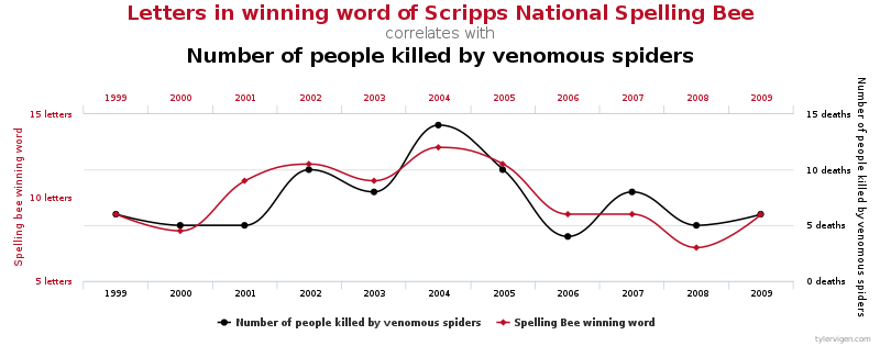
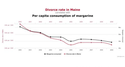
If you'd like to see more spurious correlations, click here.
A non-causal link is the information that in regions with more stork nests you have more babies. If you think that storks bring babies, this might seem logical. However, it is clearly untrue, storks do not bring the babies, and regions with more storks do not have more babies.
While a correlation tests a mere relation between two variables, a regression implies a certain theory on why two variables are related. In times of big data there is a growing amount of correlations that are hard to explain. From a theory-driven perspective, this can even be a good thing. After all, many scientific inventions were nothing short of being accidents. Likewise, through machine learning and other approaches, many patterns are found these days where we have next to no explanation to begin with. Hence, new theories even evolve out of the crunching of a lot of data, where prediction is often more important than explanation. (For more on regressions, please refer to the entry on Regression Analysis.)
Modern medicine is at the forefront of this trend, as medicine had a long tradition to have the cure in the focus of their efforts, instead of being able to explain all patterns. Modern genetics correlate specific gene sequences with potential diseases, which can be helpful, but also creates a burden or even harm. It is therefore very important to consider theory when thinking of causal relationships.
Much mischief has been done in the name of causality, while on the other hand the modern age of data made us free to be bound down by theory if we have a lot of data on our hands. Knowing the difference between the two endpoints is important, and the current scientific debate will have to move out of the muddy waters between inductive and deductive reasoning.
In this context, it should be briefly noted that a discussion about p-hacking or data dredging has evolved. The terms describe the phenomenon when scientists try to artificially improve their results or make them seem to be significant. However p-hacking becomes more widespread, there is evidence (Head et al., 2015), that it - luckily - does not distort scientific work too deeply.
To give you an idea, how hard it can be to prove a causal relationship, we recommend this video about the link of smoking and cancer.
Prediction
Statistics can be able to derive prediction based on available data. This means in general that based on the principle of extrapolation, there is enough statistical power to predict based on the available data beyond the range of the data. In other words, we have enough confidence in our initial data analysis so that we can try to predict what might happen under other circumstances, most prominently in the future, or in other places. Interpolation allows us to predict within the range of our data, spanning over gaps in the data. Hence while interpolation allows us to predict within our data, extrapolation allows prediction beyond our dataset.
Care is necessary when considering interpolation or extrapolation, as validity decreases when we dwell beyond the data we have. It takes experience to know when prediction is possible, and when it is dangerous.
1. We need to consider if our theoretical assumptions can be reasonable expanded beyond the data of our sample.
2. Our statistical model may be less applicable outside or our data range.
3. Mitigating or interacting factors may become more relevant in the space outside of our sample range.
We always need to consider these potential flaws or sources of error that may overall reduce the validity of our model when we use it for interpolation or extrapolation. As soon as we gather outside of the data space we sampled, we take the risk to produce invalid predictions. The "missing shade of blue" problem from Hume exemplifies the ambiguities that can be associated with interpolation already, and extrapolation would be seen as worse by many, as we go beyond our data sample space.
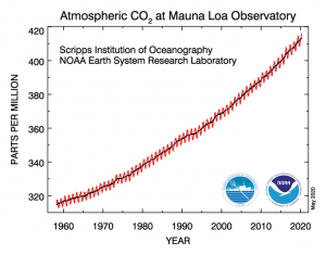
A common example of extrapolation would be a mechanistic model of climate change, where based on the trend in CO2 rates on Mauna Loa over the last decades we predict future trends. An prominent example of interpolation is the Worldclim dataset, which generates a global climate dataset based on advanced interpolation. Based on ten thousands of climate stations and millions of records this dataset provides knowledge about the average temperature and precipitation of the whole terrestrial globe. The data has been used in thousands of scientific publications and is a good example how open source data substantially enabled a new scientific arena, namely Macroecology.
Significance in regressions
P-values vs. sample size
Probability is one of the most important concepts in modern statistics. The question whether a relation between two variables is purely by chance, or following a pattern with a certain probability is the basis of all probability statistics (surprise!). In the case of linear relation, another quantification is of central relevance, namely the question how much variance is explained by the model. Between these two numbers - the amount of variance explained by a linear model, and the fact that two variables are not randomly related - are related at least to some amount. If a model is highly significant, it typically shows a high R2 value. If a model is marginally significant, then the R2 value is typically low. This relation is however also influenced by the sample size. Linear models and the related p-value describing the model are highly sensitive to sample size. You need at least a handful of points to get a significant relation, while the R2 value in this same small sample sized model may be already high. Hence the relation between sample size, R2 and p-value is central to understand how meaningful models are.
Residuals
All models are wrong, some models are useful.
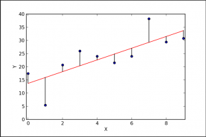
This famous sentence from Cox cannot be highlighted enough when thinking about models. In the context of residuals it comes in handy once more. Residuals are the sum (of squares) of the deviance the individual data points have from a perfectly fitted model. This is relevant for two things. First, the model assumes a perfect model. Second, reality bags to differ. Allow me to explain.
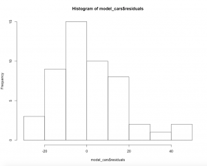
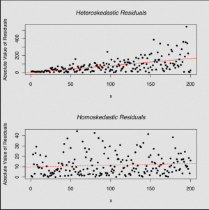
Reality is complex as people like to highlight today, but in a statistical sense that is often true. Most real datasets do not show a perfect model fit, but instead may individual data points deviate from the perfect fit the model assumes. What is now critical, is to assume that the error reflected by the residuals is normally distributed. Why, you ask? Because if it is not normally distributed, but instead shows a flawed pattern, then you missed an important variable that influences the distribution of the residuals. The distance from the points from the line should be normally distributed, which can be checked through a histogram.
What does this mean in terms of hands on inspection of the results? Just as in correlations, a scatterplot is a good first step to check out the residuals. If residuals are normally distributed, then you may realise that all errors are equally distributed across the relation. In reality, this is often not the case. Instead we often know less about one part of the data, and more about another part of the data. In addition to this we do often have a stronger relation across parts of the dataset, and a weaker understanding across other parts of the dataset. These differences are important, as they hint at underlying influencing variables or factors that we did not understand yet. Becoming versatile in reading the residuals of a linear model becomes a key skill here, as it allows you to rack biases and flaws in your dataset and analysis. This is probably the most advanced skill when it comes to reading a correlation plot.
#let's do a model for the cars data set
cars
cars<-cars
#define two variables, columnes
car_speed<-c(cars$speed)
car_dist<-c(cars$dist)

#decide on dependent and independent variable
#dependent variable = car distance
#independent variable = car speed
model_cars<-lm(car_dist~car_speed, data = cars)

#inspect residuals of the model
plot(model_cars$residuals)

#check if the model residuals follow a normal distribution
hist(model_cars$residuals)
A second case of a skewed distribution is when the residuals are showing any sort of clustering. Residuals should be distributed like stars in the sky. If they are not, then your error is not normally distributed, which basically indicates that you are missing some important information.
The third and last problem you can bump into with your residuals are gaps. Quite often you have sections in your data about which you know nothing about, as you have no data for this section. An example would be if you have a lot of height measurement of people between 140-180 cm in height, and one person that is 195 cm tall. About the section between 180-195cm we know nothing, there is a gap.
Such flaws within residuals are called errors. These errors are the reason why all models are wrong. If a model would be perfect, then there would be probably a mistake, at least when considering models in statistics. Learning to read statistical models and their respective residuals is the daily bread and butter of statistical modelling. The ability to see flaws in residuals as well as the ability to just see a correlation plot in consider the strength of the relation, if any exists, is an important skill in data mining. Learning about models means to also learn about the flaws of models.
Is the world linear?
The short answer: Mostly yes, otherwise not.
The long answer: The world is more linear than you think it is.
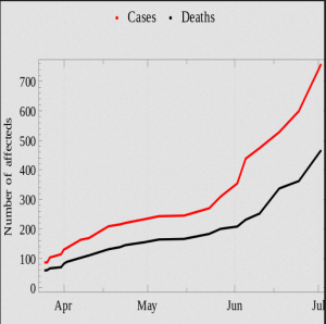
I believe that many people are puzzled by the complexity of the world, while indeed many phenomena as well as the associated underlying laws are rather simple. There are many phenomena that are linear, and this is worth noticing. People today often think that the world is non-linear. Regime shifts, disasters and crisis are thought to be prominent examples. I would argue, that even these shifts follow linear patterns, though on a smaller temporal scale. Take the last financial crisis. A lot was building up towards this crisis, yet the collapse that happened in one day followed a linear pattern, if only a strongly exponential one. Many supposably non-linear shifts are indeed linear, they just happen very quickly.
Linear patterns describe something like a natural law. Within a certain reasonable data section, you can often observe that one phenomena increases if another phenomena increases, and this relation follows a linear pattern. If you make the oven more hot, your veggies in there will be done quicker. However, this linearity only works within a certain reasonable section of the data. It would be possible to put the oven on 100 °C and the veggies would cook much slower than at 150 °C. However, this does not mean that a very long time at -30 °C in the freezer would boil your veggies in the long run as well.
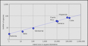
Another prominent example is the Island Theory from MacArthur and Wilson. They counted species on islands, and found out that, the larger islands are, the more species they host. While this relation has a lot of complex underpinnings, it is -on a logarithmic scale- totally linear. Larger islands contain more species, with a clearly mathematical beauty.
Phenomena that you can count are often linear on a log scale. Among coffee drinkers most coffee drinkers drink 1-2 cups per day, but few drink 10, which is probably good. Counting cup consumption per day in coffee drinker follows a log-linear distribution. The same hold for infections within an outbreak of a contagious disease. The Western African Ebola crisis was an incredibly complex and tragic event, but when we investigated the early increase in cases, the distribution is exponentially increasing -in this case-, and this increase follows an almost cruel linear pattern.
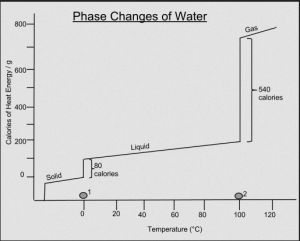
Nevertheless, there are some truly non-linear shifts, such as frost. Water is at -1 °C fundamentally different than at +1°C. This is a clear change governed by the laws of physics, yet such non-linear shifts are rare in my experience. If they occur, they are highly experimentally reproducible, and can be explained by some fundamental underlying law. Therefore, I would refrain from describing the complexity and wickedness of the modern world and its patterns and processes as non-linear. We are just not bright enough to understand the linearity in the data yet. I would advise you to seek linearity, if only logarithmic or exponential one.
References
Neuman, William Lawrence. Social Research Methods: Qualitative and Quantitative Approaches. 7. ed., Pearson new internat. ed. Pearson custom library. Harlow: Pearson, 2014.
Head, M. L., Holman, L., Lanfear, R., Kahn, A. T., & Jennions, M. D. (2015). The extent and consequences of p-hacking in science. PLoS Biology, 13 (3), e1002106. https://doi.org/10.1371/journal.pbio.1002106
Further Reading
Pearl, J., & Mackenzie, D. (2018). The book of why: The new science of cause and effect (First edition). Basic Books.
External Links
Videos
Falsificationism: A complete but understandable explanation
What is P-Hacking?: From A to izzard
Correlation doesn't equal Causation: An informative video
Proving Causality: The case of smoking and cancer
R square: What does it tell us?
Residuals: A detailed explanation
Linearity: A few words on what it is
Articles
Evidence in medicine: Some reflections on correlation and causation
Zink & the Common Cold: A helpful article
Vaccination & Autism: an enlightening article
Medical trails: A brief insight
Limits of statistics: A nice antology
Hill's Criteria of Causation: A detailed article
Spurious correlations: If you can't get enough
Regression analysis: An introduction
Correlation & Causation: Some helpful advice
What is this p-hacking discussion anyway?: Genealogy of the term
The Missing Shade of Blue: Some interesting thoughts by Hume (VPN needed)
WorldClim 2: An interesting paper on interpolation
WorldClim dataset: Global climate and weather data
Residuals: A detailed explanation
Checking residuals: Some recommendations
R square: A very detailed article
Island Theory: An example for linearity
The author of this entry is Henrik von Wehrden.

