Difference between revisions of "Wordcloud"
(Created page with "'''Note:''' This entry revolves specifically around Wordclouds. For more general information on quantitative data visualisation, please refer to Introduction to statistical...") |
m |
||
| Line 2: | Line 2: | ||
<br> | <br> | ||
__TOC__ | __TOC__ | ||
| − | + | ||
== Definition == | == Definition == | ||
Wordcloud is a cluster of words or visualisation of the most commonly or frequently used terms within the analysed data set. The basic principle is the higher the frequency, the more prominent the word on the figure is. Wordcloud is a relatively easy and quick text mining tool which allows to get a rough overview of the word usage within the dataset, which can give further ideas when studying correlations connected to word usage frequency. Wordclouds can also help get first impression of the differences or similarities when working with two textual datasets. | Wordcloud is a cluster of words or visualisation of the most commonly or frequently used terms within the analysed data set. The basic principle is the higher the frequency, the more prominent the word on the figure is. Wordcloud is a relatively easy and quick text mining tool which allows to get a rough overview of the word usage within the dataset, which can give further ideas when studying correlations connected to word usage frequency. Wordclouds can also help get first impression of the differences or similarities when working with two textual datasets. | ||
| Line 99: | Line 99: | ||
</syntaxhighlight> | </syntaxhighlight> | ||
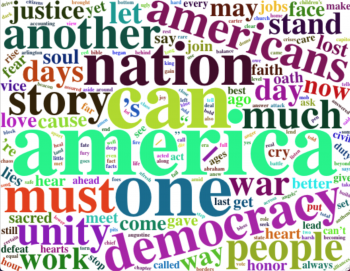
| − | [[File:BidenSpeech.png| | + | [[File:BidenSpeech.png|350px|thumb|center|Fig.1: Wordcloud of the most used words during Joe Biden's inauguration speech in 2021]] |
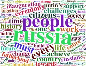
| − | [[File:PutinSpeech.png| | + | [[File:PutinSpeech.png|350px|thumb|left|Fig.1: Wordcloud of the most used words during Vladimir Putin's inauguration speech in 2016]] |
Revision as of 16:10, 5 July 2021
Note: This entry revolves specifically around Wordclouds. For more general information on quantitative data visualisation, please refer to Introduction to statistical figures. For more info on Data distributions, please refer to the entry on Data distribution.
Definition
Wordcloud is a cluster of words or visualisation of the most commonly or frequently used terms within the analysed data set. The basic principle is the higher the frequency, the more prominent the word on the figure is. Wordcloud is a relatively easy and quick text mining tool which allows to get a rough overview of the word usage within the dataset, which can give further ideas when studying correlations connected to word usage frequency. Wordclouds can also help get first impression of the differences or similarities when working with two textual datasets.
Advantages
- Due to their simple design, wordclouds rarely need additional explanation of the visualised results
- Straightforward and colourful figure can be often used for aesthetic purposes and in order to quickly get one’s point across

Disadvantages
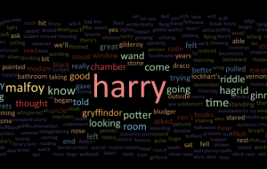
- If your data set is not prepared and cleaned you might get little to no insight into the data. Besides, it is important to have a clear idea why this method is being applied and for which purposes. Otherwise the wordcloud will simply visualise evident or common words with no use for research (Fig.1).
- General disadvantage of wordclouds is caused by the so-called “area is a bad metaphor” phenomenon. Human eyes can have difficulty visually identifying the size of an area, in this context, a word’s size compared to the other words around it. Analytical accuracy of such visualisations can be especially compromised if the words have different lengths: wordclouds tend to emphasise long words over short words as shorter words need less space and thus might appear smaller.
- Wordclouds consider one word at a time. So, for example, if customers often describe the product they purchased as “not good” in their reviews, the wordcloud will be likely to visualise it as “not” and “good” separately. Taken into account that the words are allocated randomly in the cloud, this only further impairs an accurate analysis of the visualisation.
All in all, wordclouds can be a good for intro exercise when getting familiar with text mining and neural language processing. It offers a simple and comprehensible visualisation, however its features are quite limited if a thorough textual analysis is required. As an alternative, it might be better to use a barplot or a lollipop chart, since they also make it possible to rank words by usage frequency, i.e. you can easily allocate the tenth most common word in a barplot, whereas in a wordcloud you might struggle to see the difference in sizes after identifying the first 5 most commonly used terms.
R Code
Let's try and create our own wordclouds. For the exercise we will use the transcripts of the inaugural speeches of the President of Russia (from 2016) and the President of the USA (from 2021). Creating two wordclouds can help us obtain a general understanding of which topics were in the centre of attention for the presidents during their speeches.
Before starting, we copy the text form the source and save it as a plain text with UTF-8 encoding. Once this is done, we can open our IDE to proceed with text mining.
# First we activate the necessary libraries
library(tidyverse) # loads core packages for data manipulation and functional programming
library(tm) # for text mining
library(SnowballC) # to get rid of stopwords in the text
library(wordcloud2) # to visualise as a wordcloud

x = readLines("/PresidentRussia.txt", encoding="UTF-8") #your pathway to the text file

# Transform the vector into a "list of lists" corpus for text cleaning in the next step
x = Corpus(VectorSource(x))

#Now we are ready to clean the text with the help of the SnowballC library
x = x %>%
        tm_map(removeNumbers)%>% # get rid of numbers
        tm_map(removePunctuation)%>% # get rid of punctiation
        tm_map(stripWhitespace)%>% # get rid of double spaces if present
        tm_map(content_transformer(tolower))%>% # switch words to lowercase
        tm_map(removeWords, stopwords("English"))%>% # remove stopwords in English, such as such as
                                                        #"the", "is", "at", "which", and "on".
        tm_map(removeWords,
               c("and", "the", "our", "that", "for", "will")) # remove customer stopwords

# Once we cleaned the text, we are ready to create a table with each word
# and its calculated frequency and transform it into a matrix
dtm = TermDocumentMatrix(x)
matriz = as.matrix(dtm)

# Next, we create a vector from the matrix rows with quantities and frequencies of the words
wordsvector = sort(rowSums(matriz), decreasing = TRUE)

# Now we create the final dataframe featuring two variable, word and frequency, to use for visualisation
x_df = data.frame(
        row.names = NULL,
        word = names(wordsvector),
        freq = wordsvector)

# Once this is done, here is again the whole code used above but in a form of one eloquent function
nube = function(x){

        x = Corpus(VectorSource(x))
        x = x %>%
                tm_map(removeNumbers)%>%
                tm_map(removePunctuation)%>%
                tm_map(stripWhitespace)%>%
                tm_map(content_transformer(tolower))%>%
                tm_map(removeWords, stopwords("English"))%>%
                tm_map(removeWords,
                       c("and", "the", "our", "that", "for", "will"))
        dtm = TermDocumentMatrix(x)
        matriz = as.matrix(dtm)
        wordsvector = sort(rowSums(matriz), decreasing = TRUE)
        x_df = data.frame(
                row.names = NULL,
                word = names(wordsvector),
                freq = wordsvector)
        return(x_df)
}

# Now with the help of the function which creates a clean dataframe, we just need to load the .txt file,
# run it through the function and graph the wordcloud. For the latter we are using our dataframe
# with 2 columns of words and frequency of words, with an additional setting for the size and colour of words.

#Fig.2
Putin = readLines("/PresidentRussia.txt", encoding = "UTF-8")
df_putin = nube(Putin)
wordcloud2(data = df_putin[1:2], size = 0.8, color = 'random-dark')


# For comparison we can also look at the inaugural speech of US President Joe Biden from 2021
# Fig.3
Biden = readLines("/PresidentUS.txt", encoding = "UTF-8")
df_biden = nube(Biden)
wordcloud2(data = df_biden[1:2], size = 0.8, color = 'random-dark')
References and further reading material
The code was inspied by
- Easy word cloud with R — Peru’s presidential debate version by Ana Muñoz Maquera
- "My First Data Science Project: A Word Cloud Comparing the 2020 Presidential Debates" by Tori White
Further sources
- The official transcript of the inaugural speech of the President of Russian (2016)
- Inaugural Address by President Joseph R. Biden, Jr. (2021)
- Guide to the Wordcloud2
The author of this entry is Olga Kuznetsova.

