Simple Statistical Tests
| Method categorization | ||
|---|---|---|
| Quantitative | Qualitative | |
| Inductive | Deductive | |
| Individual | System | Global |
| Past | Present | Future |
In short: Simple statistical tests encapsule an array of simple statistical tests that are all built on probability, and no other validation criteria.
Background
Simple statistical tests statistics provide the baseline for advanced statistical thinking. While they are not so much used today within empirical analysis, simple tests are the foundation of modern statistics. The student t-test which originated around 100 years ago provided the crucial link from the more inductive thinking of Sir Francis Bacon towards the testing of hypotheses and the actual statistical testing of hypotheses. The formulation of the so-called null hypothesis is the first step within simple tests. Informed from theory this test calculates the probability whether the sample confirms the hypothesis or not. Null hypotheses are hence the assumptions we have about the world, and these assumptions can be confirmed or rejected.
The following information on simple statistical tests assumes some knowledge about data formats and data distribution. If you want to learn more about these, please refer to the entries on Data formats and Data distribution.
Most relevant simple tests
One sample t-test
The easiest example is the one sample t-test: it allows us to test a dataset (more specifically, its mean value) versus a specified value. For this purpose, the t-test gives you a p-value at the end. If the p-value is below 0.05, the sample differs significantly from the reference value. Important: The data of the sample(s) has to be normally distributed.
Example: Do the packages of your favourite cookie brand always contain as many cookies as stated on the outside of the box? Collect some of the packages, weigh the cookies contained therein and calculate the mean weight. Now, you can compare this value to the weight that is stated on the box using a one sample t-test.
For more details and R examples on t-tests, please refer to the T-Test entry.
Two sample t-test
Two sample tests are the next step. These allow a comparison of two different datasets within an experiment. They tell you if the means of the two datasets differ significantly. If the p-value is below 0,05, the two datasets differ significantly. It is clear that the usefulness of this test widely depends on the number of samples - the more samples we have for each dataset, the more we can understand about the difference between the datasets.
Important: The data of the sample(s) has to be normally distributed. Also, the kind of t-test you should apply depends on the variance in the parent populations of the samples. For a Student’s t-test, equal variances in the two groups are required. A Welch t-test, by contrast, can deal with samples that display differing variances (1). To know whether the datasets have equal or varying variances, have a look at the F-Test.
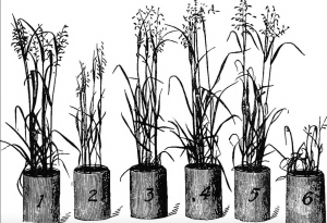
Example: The classic example would be to grow several plants and to add fertiliser to half of them. We can now compare the gross of the plants between the control samples without fertiliser and the samples that had fertiliser added.
Plants with fertiliser (cm): 7.44 6.35 8.52 11.40 10.48 11.23 8.30 9.33 9.55 10.40 8.36 9.69 7.66 8.87 12.89 10.54 6.72 8.83 8.57 7.75
Plants without fertiliser (cm): 6.07 9.55 5.72 6.84 7.63 5.59 6.21 3.05 4.32 8.27 6.13 7.92 4.08 7.33 9.91 8.35 7.26 6.08 5.81 8.46
The result of the two-sample t-test is a p-value of 7.468e-05, which is close to zero and definitely below 0,05. Hence, the samples differ significantly and the fertilizer is likely to have an effect.
For more details on t-tests, please refer to the T-Test entry.
| ExpandExpand here for an R example for two-sample t-Tests. |
|---|
Paired t-test
Paired t-tests are the third type of simple statistics. These allow for a comparison of a sample before and after an intervention. Within such an experimental setup, specific individuals are compared before and after an event. This way, the influence of the event on the dataset can be evaluated. If the sample changes significantly, comparing start and end state, you will receive again a p-value below 0,05.
Important: for the paired t-test, a few assumptions need to be met.
- Differences between paired values follow a normal distribution.
- The data is continuous.
- The samples are paired or dependent.
- Each unit has an equal probability of being selected
Example: An easy example would be the behaviour of nesting birds. The range of birds outside of the breedig season dramatcally differs from the range when they are nesting.
For more details on t-tests, please refer to the T-Test entry.
| ExpandExpand here for an R example on paired t-tests. |
|---|
Chi-square Test of Stochastic Independence
The Chi-Square Test can be used to check if one variable influences another one, or if they are independent of each other. The Chi Square test works for data that is only categorical.
Example: Do the children of parents with an academic degree visit a university more often, for example because they have higher chances to achieve good results in school? The table on the right shows the data that we can use for the Chi-Square test.
For this example, the chi-quare test yields a p-value of 2.439e-07, which is close to zero. We can reject the null hypothesis that there is no dependency, but instead assume that, based on our sample, the education of parents has an influence on the education of their children.
| ExpandExpand here for an R example for the Chi-Square Test. |
|---|
Wilcoxon Test
The next important test is the Wilcoxon rank sum test. This test is also a paired test. What is most relevant here is that not the real numbers are introduced into the calculation, but instead these numbers are transformed into ranks. In other words, you get rid of the question about normal distribution and instead reduce your real numbers to an order of numbers. This can come in handy when you have very skewed distribution - so a exceptionally non-normal distribution - or large gaps in your data. The test will tell you if the means of two samples differ significantly (i.e. p-value below 0,05) by using ranks.
Example: An example would be the comparison in growths of young people compared to their size as adults. Imagine you have a sample where half of your people are professional basketball players then the real size of people would not make sense. Therefore, as a robust measure in modern statistics, rank tests were introduced.
| ExpandExpand here for an R example for the Wilcoxon Test. |
|---|
f-test
The f-test allows you to compare the variance of two samples. Variance is calculated by taking the average of squared deviations from the mean and tells you the degree of spread in your data set. The more spread the data, the larger the variance is in relation to the mean. If the p-value of the f-test is lower than 0,05, the variances differ significantly. Important: for the f-Test, the data of the samples has to be normally distributed.
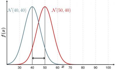
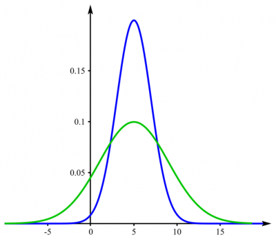
Example: If you examine players in a basketball and a hockey team, you would expect their heights to be different on average. But maybe the variance is not. Consider Figure 1 where the mean is different, but the variance the same - this could be the case for your hockey and basketball team. In contrast, the height could be distributed as shown in Figure 2. The f-test then would probably yield a p-value below 0,05.


| ExpandExpand here for an R example for the f-Test. |
|---|
Normativity & Future of Simple Tests
Simple tests are not abundantly applied these days in scientific research, and often seem outdated. Much of the scientific designs and available datasets are more complicated than what we can do with simple tests, and many branches of sciences established more complex designs and a more nuanced view of the world. Consequently, simple tests grew kind of out of fashion.
However, simple tests are not only robust, but sometimes still the most parsimonious approach. In addition, many simple tests are a basis for more complicated approaches, and initiated a deeper and more applied starting point for frequentist statistics.
Simple tests are often the endpoint of many introductionary teachings on statistics, which is unfortunate. Overall, their lack in most of recent publications as well as wooden design frames of these approaches make these tests an undesirable starting point for many students, yet they are a vital stepping stone to more advanced models.
Hopefully, one day school children will learn simple test, because they could, and the world would be all the better for it. If more people early on would learn about probability, and simple tests are a stepping stone on this long road, there would be an education deeper rooted in data and analysis, allowing for better choices and understanding of citizens.
Key Publications
- Student" William Sealy Gosset. 1908. The probable error of a mean. Biometrika 6 (1). 1–25.
- Cochran, William G. 1952. The Chi-square Test of Goodness of Fit. The Annals of Mathematical Statistics 23 (3). 315–345.
- Box, G. E. P. 1953. Non-Normality and Tests on Variances. Biometrika 40 (3/4). 318–335.
References
(1) Article on the "Student's t-test" on Wikipedia
Further Links
- Videos
The Hypothesis Song: A little musical introduction to the topic
Hypothesis Testing: An introduction of the Null and Alternative Hypothesis
The Scientific Method: The musical way to remember it
Popper's Falsification: The explanation why not all swans are white
Type I & Type II Error: A quick explanation
Validity: An introduction to the concept
Reliability: A quick introduction
The Confidence Interval: An explanation with vivid examples
Choosing which statistical test to use: A very detailed videos with lots of examples
One sample t-test: An example calculation
Two sample t-test: An example calculation
Introduction into z-test & t-test: A detailed video
Chi-Square Test: Example calculations from the world of e-sports
F test: An example calculation
- Articles
History of the Hypothesis: A brief article through the history of science
The James Lind Initiative: One of the earliest examples for building hypotheses
The Scientific Method: A detailed and vivid article
Falsification: An introduction to Critical Rationalism (German)
Statistical Validity: An overview of all the different types of validity
Reliability & Validity: An article on their relationship
Statistical Reliability: A brief article
Reliability Analysis: An overview about different approaches
How reliable are the Social Sciences?: A short article by The New York Times
Uncertainty, Error & Confidence: A very long & detailed article
Student t-test: A detailed summary
One sample t-test: A brief explanation
Two sample t-test: A short introduction
Paired test: A detailed summary
Chi-Square Test: A vivid article
Wilcoxon Rank Sum Test: A detailed example calculation in R
F test: An example in R
The authors of this entry are Henrik von Wehrden and Carlo Krügermeier.


