Dummy variables
In short: A dummy variable is a variable that is created in regression analysis to represent a given qualitative variable through a quantitative one, which takes one of two values: zero or one. It is needed to make algorithm calculations possible, since they always rely on numeric values. The entry further provides code for both, R and Python programming languages.
This entry focuses on the dummy variables and the way they can be encoded with the help of R and Python programming languages to be further used for regression analysis. For more information on regression, please refer to the entry on Regression Analysis. To see more examples of dummy variables applied, please refer to the Price Determinants of Airbnb Accommodations and Likert Scale entries.
Contents
Dummy variables
A dummy variable is a variable that is created in regression analysis to represent a given qualitative variable through a quantitative one, which takes one of two values: zero or one.
Typically we use quantitative variables for linear regression model equations. These can be a specific size of an object, age of an individual, population size, etc. But sometimes the predictor variables can be qualitative. Those are variables that do not have a numeric value associated with them, e.g. gender, country of origin, marital status. Since machine learning algorithms including regression rely on numeric values, these qualitative values have to be converted.
Some qualitative variables have a natural idea of order and can be easily converted to a numeric value accordingly, e.g. number of the month instead of its name, such as 3 instead of “March”. But it is not possible for nominal variables. However, this can be a common trap when preparing one’s dataset for the regression analysis. For the linear model converting ordinal values to numeric ones would not make much sense, as the model assumes the change between each value to be constant. What is usually done instead is a series of binary variables to capture the different levels of the qualitative variable.
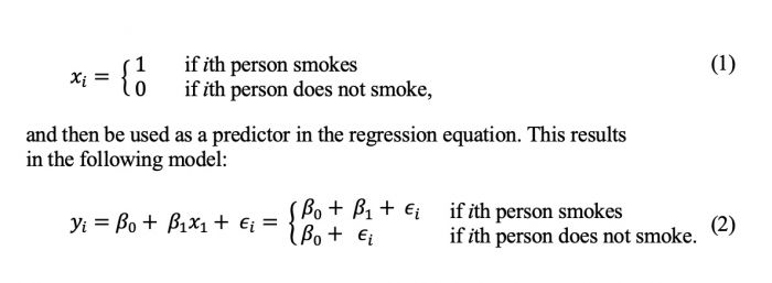
If the qualitative variable, which is also known as a factor, has only two levels, then integrating it into a regression model is very simple: we need to use dummy variables. For example, our variable can describe if a given individual smokes or does not:
If a qualitative variable has more than two levels, a single dummy variable cannot represent all possible values. In this case we create additional dummy variables. The general rule that applies here, is the following: If you have k unique terms, you use k - 1 dummy variables to represent.
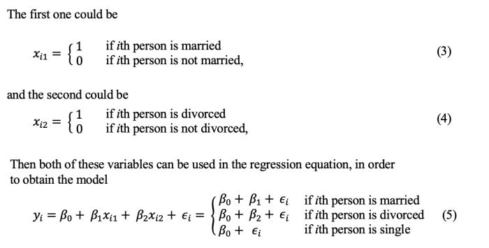
Let’s consider a variable representing one’s marital status. Possible values are “single”, “divorced” or “married”. In this case we create two dummy variables.
If, for example, our model helps us predict an individual’s average insurance rate, then β0 can be interpreted as the average insurance rate for a single person, β1 can be interpreted as the difference in the average insurance rate between a single person and a married one, and β2 can be interpreted as the difference in the average insurance rate between a single person and a divorced one. As mentioned before, there will always be one fewer dummy variable than the number of levels. Here, the level with no dummy variable is “single”, also known as the baseline.
How to encode dummy variables in R/Python
Converting a single column of values into multiple columns of binary values, or dummy variables, is also known as “one-hot-encoding”. Not all machines know how to convert qualitative variables into dummy variables automatically, so it is important to know different methods how to do it yourself. We will look at different ways to code it with the help of both, R and Python programming languages. The dataset "ClusteringHSS.csv" used in the following examples can be downloaded from Kaggle.
R-Script
library(readr) # for the dataset importing

data <- read_csv("YOUR_PATHNAME")

head(data)
#Output:
# A tibble: 6 x 5
#     ID Gender_Code Region Income Spending
#  <dbl> <chr>       <chr>   <dbl>    <dbl>
#1     1 Female      Rural      20       15
#2     2 Male        Rural       5       12
#3     3 Female      Urban      28       18
#4     4 Male        Urban      40       10
#5     5 Male        Urban      42        9
#6     6 Male        Rural      13       14

summary(data) # Two variables are categorical, gender and region
              # We see that our dataframe has some NAs in the Income and Spending columns
#Output:
#       ID       Gender_Code           Region              Income         Spending
# Min.   :   1   Length:1113        Length:1113        Min.   : 5.00   Min.   : 5.00
# 1st Qu.: 279   Class :character   Class :character   1st Qu.:14.00   1st Qu.: 7.00
# Median : 557   Mode  :character   Mode  :character   Median :25.00   Median :10.00
# Mean   : 557                                         Mean   :26.02   Mean   :11.28
# 3rd Qu.: 835                                         3rd Qu.:37.00   3rd Qu.:15.00
# Max.   :1113                                         Max.   :50.00   Max.   :20.00
#                                                      NA's   :6       NA's   :5


data <- na.omit(data) # Apply na.omit function to delete the NAs
summary(data)         # Printing updated data. No NAs

#Let's look at the possible values within each variable
unique(data$Gender_Code)
#Output: [1] "Female" "Male" -> binary
unique(data$Region)
#Output: [1] "Rural" "Urban" -> binary

#OPTION 1
#create dummy variables manually. k = k-1
Gender_Code_Male <- ifelse(data$Gender_Code == 'Male', 1, 0) #if male, gender equals 1, if female, gender equals 0.
Region_Urban <- ifelse(data$Region == 'Urban', 1, 0) #if urban, region equals 1, if rural, region equals 0.

#create data frame to use for regression
data <- data.frame(ID = data$ID,
                       Gender_Code_Male = Gender_Code_Male,
                       Region_Urban = Region_Urban,
                       Income = data$Income,
                       Spending = data$Spending)
#view data frame
data

#Output:
#     ID Gender_Code_Male Region_Urban Income Spending
#1     1                0            0     20       15
#2     2                1            0      5       12
#3     3                0            1     28       18
#4     4                1            1     40       10
#5     5                1            1     42        9
#(...)


#OPTION 2
#Using the fastDummies Package
# Install and import fastDummies:
install.packages('fastDummies')
library('fastDummies')

data <- read_csv("YOUR_PATHNAME") #prepare the data frame again if needed
data <- na.omit(data)

# Make dummy variables of two columns and remove the previous columns with categorical values:
data <- dummy_cols(data, select_columns = c('Gender_Code', 'Region'), remove_selected_columns = TRUE)

#view data frame
data
#Output:
# A tibble: 1,090 x 7
#      ID Income Spending Gender_Code_Female Gender_Code_Male Region_Rural Region_Urban
#   <dbl>  <dbl>    <dbl>              <int>            <int>        <int>        <int>
# 1     1     20       15                  1                0            1            0
# 2     2      5       12                  0                1            1            0
# 3     3     28       18                  1                0            0            1
# 4     4     40       10                  0                1            0            1
# 5     5     42        9                  0                1            0            1


# CREATING A LINEAR MODEL
# In our multiple regression linear model we will try to predict the income based on
# other variables given in our data set.
# In the formula we drop the Gender_Code_Female and Region_Rural to avoid singularity error,
# as they have an exact linear relationship with their counterparts.
model <- lm(Income ~ Spending + Gender_Code_Male + Region_Urban,
            data = data)

summary(model)

#Call:
#lm(formula = Income ~ Spending + Gender_Code_Male + Region_Urban,
#    data = data)
#
#Residuals:
#     Min       1Q   Median       3Q      Max
#-13.1885  -6.1105  -0.1535   5.8825  12.9356
#
#Coefficients:
#                 Estimate Std. Error t value Pr(>|t|)
#(Intercept)      14.06584    0.63227  22.246   <2e-16 ***
#Spending          0.02634    0.04577   0.575   0.5651
#Gender_Code_Male  0.83435    0.42116   1.981   0.0478 *
#Region_Urban     22.78781    0.42049  54.193   <2e-16 ***
#---
#Signif. codes:  0 ‘***’ 0.001 ‘**’ 0.01 ‘*’ 0.05 ‘.’ 0.1 ‘ ’ 1
#
#Residual standard error: 6.927 on 1086 degrees of freedom
#Multiple R-squared:  0.7319,	Adjusted R-squared:  0.7312
#F-statistic: 988.5 on 3 and 1086 DF,  p-value: < 2.2e-16
The fitted regression line turns out to be:
Income = 14.06584 + 0.02634*(Spending) + 0.83435*(Gender_Code_Male) + 22.78781*(Region_Urban)
We can use this equation to find the estimated income for an individual based on their monthly spendings, gender and region. For example, an individual who is a female living in the rural area and spending 5 mln per month is estimated to have an income of 14.19754 mln per month:
Income = 14.06584 + 0.02634*5 + 0.83435*0 + 22.78781*0 = 14.19754
Python Script
import pandas as pd # for data manipulation
import statsmodels.api as sm # for statistical computations and models

df = pd.read_csv("YOUR_PATHNAME")

#Let's look at our data.
#We have five variables and 1112 entries in total
df

#        ID Gender_Code Region  Income  Spending
#0        1      Female  Rural    20.0      15.0
#1        2        Male  Rural     5.0      12.0
#2        3      Female  Urban    28.0      18.0
#3        4        Male  Urban    40.0      10.0
#4        5        Male  Urban    42.0       9.0
#    ...         ...    ...     ...       ...
#1108  1109      Female  Urban    33.0      16.0
#1109  1110        Male  Urban    48.0       7.0
#1110  1111        Male  Urban    31.0      16.0
#1111  1112        Male  Urban    50.0      14.0
#1112  1113        Male  Urban    26.0      11.0
#[1113 rows x 5 columns]


df.info()           # Two variables are categorical, Gender_Code and Region
#<class 'pandas.core.frame.DataFrame'>
#RangeIndex: 1113 entries, 0 to 1112
#Data columns (total 5 columns):
# #   Column       Non-Null Count  Dtype
#---  ------       --------------  -----
# 0   ID           1113 non-null   int64
# 1   Gender_Code  1107 non-null   object
# 2   Region       1107 non-null   object
# 3   Income       1107 non-null   float64
# 4   Spending     1108 non-null   float64
#dtypes: float64(2), int64(1), object(2)

df.isnull().sum()   # We see that our dataframe has some NAs in every variable except for ID
#ID             0
#Gender_Code    6
#Region         6
#Income         6
#Spending       5
#dtype: int64

df = df.dropna() # Apply na.omit function to delete the
df.info()        # No NAs

pd.unique(df.Gender_Code)
# Output: array(['Female', 'Male'], dtype=object) -> The variable is binary

pd.unique(df.Region)
# Output: array(['Rural', 'Urban'], dtype=object) -> The variable is binary


#OPTION 1
# using .map to create dummy variables
# dataframe['category_name'] = df.Category.map({'unique_term':0, 'unique_term2':1})
df['Gender_Code_Male'] = df.Gender_Code.map({'Female':0, 'Male':1})
df['Region_Urban'] = df.Region.map({'Rural':0, 'Urban':1})

#drop the categorical columns that are no longer useful
df.drop(['Gender_Code', 'Region'], axis=1, inplace=True)
#view data frame
df.head()
#   ID  Income  Spending  Gender_Code_Male  Region_Urban
#0   1    20.0      15.0                 0             0
#1   2     5.0      12.0                 1             0
#2   3    28.0      18.0                 0             1
#3   4    40.0      10.0                 1             1
#4   5    42.0       9.0                 1             1

#OPTION 2
#Using the pandas.get_dummies function.
# Create dummy variables for multiple categories
# drop_first=True handles the k - 1 rule
df = pd.get_dummies(df, columns=['Gender_Code', 'Region'], drop_first=True)
# this drops original Gender_Code and Region columns
# and creates dummy variables

#view data frame
df.head()
#   ID  Income  Spending  Gender_Code_Male  Region_Urban
#0   1    20.0      15.0                 0             0
#1   2     5.0      12.0                 1             0
#2   3    28.0      18.0                 0             1
#3   4    40.0      10.0                 1             1
#4   5    42.0       9.0                 1             1


#CREATING A LINEAR MODEL
# with statsmodels
# Setting the values for independent (X) variables (what we use for prediction)
# and dependent (Y) variable (what we want to predict).

x = df[['Spending', 'Gender_Code_Male', 'Region_Urban']]
y = df['Income']

x = sm.add_constant(x)  # adding a constant, or the intercept

model = sm.OLS(y, x).fit()
predictions = model.predict(x)

print_model = model.summary()
print(print_model)

#                            OLS Regression Results
#==============================================================================
#Dep. Variable:                 Income   R-squared:                       0.732
#Model:                            OLS   Adj. R-squared:                  0.731
#Method:                 Least Squares   F-statistic:                     988.5
#Date:                Mon, 19 Sep 2022   Prob (F-statistic):          7.50e-310
#Time:                        15:24:54   Log-Likelihood:                -3654.3
#No. Observations:                1090   AIC:                             7317.
#Df Residuals:                    1086   BIC:                             7337.
#Df Model:                           3
#Covariance Type:            nonrobust
#====================================================================================
#                       coef    std err          t      P>|t|      [0.025      0.975]
#------------------------------------------------------------------------------------
#const               14.0658      0.632     22.246      0.000      12.825      15.306
#Spending             0.0263      0.046      0.575      0.565      -0.063       0.116
#Gender_Code_Male     0.8343      0.421      1.981      0.048       0.008       1.661
#Region_Urban        22.7878      0.420     54.193      0.000      21.963      23.613
#==============================================================================
#Omnibus:                      535.793   Durbin-Watson:                   1.977
#Prob(Omnibus):                  0.000   Jarque-Bera (JB):               59.649
#Skew:                           0.042   Prob(JB):                     1.12e-13
#Kurtosis:                       1.857   Cond. No.                         39.2
#==============================================================================
#Notes:
#[1] Standard Errors assume that the covariance matrix of the errors is correctly specified.
The fitted regression line turns out to be:
Income = 14.0658 + 0.0263*(Spending) + 0.8343*(Gender_Code_Male) + 22.7878*(Region_Urban)
We can use this equation to find the estimated income for an individual based on their monthly spendings, gender and region. For example, an individual who is a female living in the rural area and spending 5 mln per month is estimated to have an income of 14.1973 mln per month:
Income = 14.0658 + 0.0263*5 + 0.8343*0 + 22.7878*0 = 14.1973
Useful sources
The author of this entry is Olga Kuznetsova.

