Bayesian Inference

Method Categorisation:
Quantitative - Qualitative
Deductive - Inductive
Individual - System - Global
Past - Present - Future

In short: Bayesian Inference is a statistical line of thinking that derives calculations based on distributions derived from the currently available data.

Background

SCOPUS hits per year for Bayesian Inference until 2020. Search terms: 'Bayesian' in Title, Abstract, Keywords. Source: own.

The basic principles behind Bayesian methods can be attributed to the probability theorist and philosopher, Thomas Bayes. His method was published posthumously by Richard Price in 1763. While at the time, the approach did not gain that much attention, it was also rediscovered and extended upon independently by Pierre Simon Laplace (1). Bayes' name only became associated with the method in the 1900s (3).

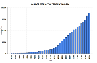
The family of methods based on the concept of Bayesian analysis has risen the last 50 years alongside the increasing computing power and the availability of computers to more people, enabling the technical precondition for these calculation-intense approaches. Today, Bayesian methods are applied in a various and diverse parts of the scientific landscape, and are included in such diverse approaches as image processing, spam filtration, document classification, signal estimation, simulation, etc. (2, 3)

What the method does

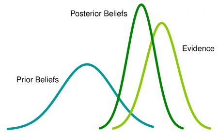
Bayesian analysis relies on using probability figures as an expression of our beliefs about events. Consequently, assigning probability figures to represent our ignorance about events is perfectly valid in Bayesian approach. The probabilities, hence, depend on the current knowledge we have on the event that we are setting our belief on; the initial belief is known is "prior", and the probability figure assigned to the prior is called "prior probability". Initially, these probabilities are essentially subjective, as these priors are not the properties of a larger sample. However, the probability figure is updated as we receive more data. The final probabilities that we get after applying the Bayesian analysis, called "posterior probability", is based on our prior beliefs about the hypothesis, and the evidence that we collect:

The probability distribution for prior, evidence, and posterior.

So, how do we update the probability, and hence our belief about the event, as we receive new information? This is achieved using Bayes' Theorem.

Bayes' Theorem

Bayes theorem provides a formal mechanism for updating our beliefs about an event based on new data. However, we need to establish some definitions before being able to understand and use Bayes' theorem.

Conditional Probability is a probability based on some background information. If we consider two events A and B, conditional probability can be represented as:

   P(A|B)

This representation can be read as the probability of event A occurring (or being observed) given that event B occurred (or B was observed). Note that in this representation, the order of A and B matters. Hence P(A|B) and P(B|A) are convey different information (discussed in the coin-toss example below).

Joint Probability, also called "conjoint probability", represents the probability of two events being true - i.e. two events occuring - at the same time. If we assume that the events A and B are independent, this can be represented as:

   P(A\ and\ B)=P(B\ and\ A)= P(A)P(B)

Interestingly, the conjoint probability can also be represented as follows:

   P(A\ and\ B) = P(A)P(B|A)

   P(B\ and\ A) = P(B)P(A|B)

Marginal Probability is just the probability for one event of interest (e.g. probability of A regardless of B or probability of B regardless of A) and can be represented as follows. For the probability of event E:

   P(E)

Technically, these are all the things that we need to be able to piece together the formula that you see when you search for "Bayes theorem" online.

   P(A\ and\ B) = P(B\ and\ A)

Caution: Even though p(A and B) = p(B and A), p(A|B) is not equal to p(B|A).

We can now replace the two terms on the side with the alternative representation of conjoint probability as shown above. We get:

   P(B)P(A|B)=P(A)P(B|A)

   P(A|B) = \frac{P(B|A)*(A)}{P(B)}

Note: the marginal probability `p(B)` can also be represented as:

   P(B) = P(B|A)*P(A) + P(B|not\ A)*P(not\ A)

We can see all three definitions that were discussed above appearing in the latter two formulae above. Now, let's see how this formulation of Bayes' Theorem can be applied in a simple coin toss example:

Example I: Classic coin toss

Imagine, you are flipping 2 fair coins. The outcome of one of the coins was a Head. Given that you already got a Head, what is the probability of getting another Head?

(This is same as asking: what is the probability of getting 2 Heads given that you know you have at least one Head)

Solution: If we represent the outcome of Heads by a H and the outcome of Tails by a T, then the possible outcomes of the two coins being tossed simultaneously can be written as: `HH`, `HT`, `TH`, `TT`

The two events A, and B are:

A = the outcome is 2 heads (also called "prior probability")

B = one of the outcomes was a head (also called "marginal probability")

So, essentially, the problem can be stated as: what is the probability of getting 2 heads, given that we've already gotten 1 head? This is the posterior probability, which can be represented mathematically as:

   P(2\ heads|1\ head)

In this case, the prior probability is the probability of getting 2 heads. We can see from our representation above that the prior probability is 1/4 as there is only one outcome where there are 2 Heads.

Similarly, the likelihood is the probability of getting at least 1 Head given that we get 2 Heads; think of likelihood as being similar to posterior probability, with the two events switched. If we get 2 Heads, then the probability of getting 1 Head is 100%. Hence, the likelihood is 1.

Finally, we need to know what the probability of getting at least 1 Head, the marginal, is. In this example, there are three cases where the outcome is at least 1 Head. Hence, the marginal is 3/4.

We saw above that the formula for Bayes' Theorem looks like:

   P(A|B) = \frac{P(B|A)*(A)}{P(B)}

We can represent the formula above in context of this case with the following:

   P(2\ heads|1\ head) = \frac{P(1\ head|2\ heads)* P(2\ heads)}{P(1\ head)}
   = \frac{1 * \frac{1}{4}}{\frac{3}{4}}
   = \frac{1}{3}

Since this is a toy example, it is easy to come up with all the probabilities we need. However, in real world, we might not be able to pin down the exact probability and likelihood values as easily as we did here.

Using Bayes' Theorem to Update Our Beliefs

What we discussed earlier captures one use-case scenario of Bayes' Theorem. However, we already established that Bayes' Theorem allows us to systematically update our beliefs, or hypothesis, about events as we receive new data. This is called the **diachronic interpretation** of Bayes' Theorem.

To make things a bit easier to understand in this line of thinking, one way of making this formulation a bit easier to understand is by replacing the As and Bs that we have been using until now with **hypothesis (H)**/belief and **data (D)** respectively (however, the As and Bs don't necessarily need to be that):

   P(hypothesis|data) = \frac{P(hypothesis)*P(data|hypothesis)}{P(data)}

This formula can be parsed as follows:

Let's go through this formula from the left side to right:

Posterior Probability is the probability that we are interested in. We want to establish if our belief is consistent given the data that we have been able to acquire/observe.
Prior Probability is the probability of the belief before we see any data. This is usually based on the background information that we have about the nature of distribution that the samples come from, or past events. This can be computed based on historical data sets or be selected by domain experts on a subject matter.
Likelihood is the probability of the data under the hypothesis.
The Marginal above is a normalizing constant which represents the probability of the data under any hypothesis.

There are two key assumptions that are made about hypotheses here: 1. Hypotheses are mutually exclusive - at most one hypothesis can be true. 2. Hypotheses are collectively exhaustive - assuming any given hypothesis being considered comes from a pool of hypotheses, at least one of the hypotheses in the pool has to be true.

Example II: Monty Hall Problem

(This example is largely based on the book "Think Bayes" by Allan B. Downey (referenced below))

The Monty Hall problem is based on the famous show called "Let's Make a Deal" where Monty Hall was the host. In one of the games on the show, Monty would present the following problem to the contestant:

There are three doors (Door 1, Door 2, and Door 3). Behind two of those doors are worthless items (a goat), and behind one of the door is something valuable (a car). You don't know what is behind which door, but Monty knows.

You are asked to choose one of the doors. Then, Monty opens one of the 2 remaining doors. He only ever opens the door with a goat behind it.

Let's say you choose Door 1 - there is no goat behind Door 1, you are lucky. Then Monty will open either Door 2 or Door 3. Whichever door he opens will contain a goat in it. Then you are asked if you want to change your decision and switch to a different door.

The question that has baffled people over the years is: "Do you stick to your choice or do you switch?" While there are many ways to look at this problem, we could view this from a Bayesian perspective, and later verify if this is correct with an experiment.

Step 1: Let's summarize the problem in a more mathematical way:

Initially, we don't know anything so we choose Door 1:

Hypothesis (H): Door 1 has a car behind it.

Then, Monty opens a door. This changes our knowledge about the system.

Data (D): Monty has revealed a door with a goat behind it.

What is the probability that Door 1 has a car behind it?

Problem:

   P(H|D) = ?

Step 2: Now, let's summarize our knowledge. We use the Bayes' Theorem to solve this problem:

   P(H|D) = \frac{P(D|H)*P(H)}{P(D)}

This can be represented as the following:

   P(H|D) = \frac{P(D|H)*P(H)}{P(D|H)*P(H) + P(D|not\ H)*P(not\ H)}

Initial probability of the Hypothesis being true (prior):

   P(H) = 1/3

Similarly:

   P(not\ H) = 1 - P(H) = 1 - \frac{1}{3} = \frac{2}{3}

So, what is `P(D|H)`? This is the probability that Monty opens a door with a goat behind it given that the car is behind Door 1 (the door that we initially choose). Since Monty always opens a door with a goat behind it, this probability is 1. So,

   P(D|H) = 1

What is `P(D|not H)`? This is the probability that Monty opens a door with a goat behind it given that the goat is not behind Door 1. Again, since Monty always opens a door with a goat behind it anyway, this probability is also 1. So,

   P(D|not\ H) = 1

Step 3: Now, we have all the information we need to solve this problem the Bayesian way:

   P(H|D) = \frac{P(D|H)*P(H)}{P(D|H)*P(H) + P(D|not\ H)*P(not\ H)}
   P(H|D) = \frac{1 * 1/3}{(1*1/3)+(1 * 2/3)}
   P(H|D) = 1/3

Conclusion: So, the probability that your hypothesis (or rather belief) that the car is behind the door you choose (Door 1) is only `1/3`. Conversely, the probability that the the car is behind a door that you did not choose is `2/3`.

How can we use this to guide our decision? Since the probability that the car is behind a door that we have not chosen `2/3` and Monty has already opened one door with a goat behind it, it would make more sense to switch.

Using Bayes' Theorem, we could reach this conclusion purely analytically.

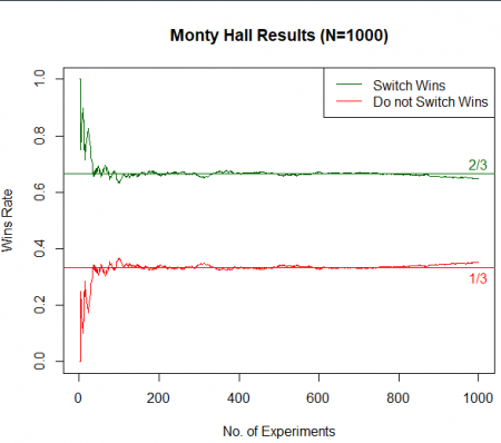
In addition, we can verify the fact that over time the strategy of switching the doors when asked wins 2/3 of the time:

R Script for the Monty Hall example

If you want to verify this experimentally, you are encouraged to run the following R script to see the results:

1. 1. 1. Function that Plays the Monty Hall Problem ####

monty_hall <- function(){

 # 1. Available doors
 door_options <- c(1, 2, 3)
 
 # 2. The door selected by the player initially.
 selected_door <- sample(1:3, size=1)
 
 # 3. The door which contains a car behind it.
 winning_door <- sample(1:3, size=1)

 if (selected_door==winning_door){
   # remove the selected door from door options
   door_options = setdiff(door_options, selected_door)
   
   # The door that Monty opens
   open_door = sample(door_options, size=1)
   
   # The remaining door (player wins if they don't switch)
   switching_door = setdiff(door_options, open_door)
 }
 else{
   # Remove the selected door from door options
   door_options = setdiff(door_options, selected_door)
   
   # Remove the winning door from door options
   door_options = setdiff(door_options, winning_door)
   
   # Select the open door
   open_door = door_options
   
   # If player switches, they will switch to the winning door
   switching_door = winning_door
 }
 
 # If player switches and lands to the winning door,
 #  "switching strategy" wins this round
 if (switching_door == winning_door){
   switch = 1
   non_switch = 0
 }
 # If player selected the winning door and sticks to it,
 # "non-switching strategy" wins this round 
 else{
   switch = 0
   non_switch = 1
 }

 return(c("switch_wins"=switch, "non_switch_wins"=non_switch))

}

1. 1. 1. Investigation on wins and losses over time ####

N = 1000 # No. of experiments

Vectors used to store rate of wins of each strategy at each experiment step

switching_wins_rate <- c() non_switching_wins_rate <- c() switching_wins <- c() non_switching_wins <- c()

Conduct the experiments

for (i in 1:N) {

 set.seed(i) # change seed for each experiment
 result <- monty_hall()
 # store the wins and losses
 switching_wins <- c(switching_wins, result[1])
 non_switching_wins <- c(non_switching_wins, result[2])
 # calculate winning rate based on current and past experiments
 total <- sum(switching_wins) + sum(non_switching_wins)
 swr <- sum(switching_wins) / total
 nswr <- sum(non_switching_wins) / total
 # store the winning rate of 2 strategies in the vectors
 # defined above 
 switching_wins_rate <- c(switching_wins_rate, swr)
 non_switching_wins_rate <- c(non_switching_wins_rate, nswr)

}

Plot the result of the experiments

plot(switching_wins_rate,

    type="l",
    col="darkgreen", cex=1.5,
    ylim=c(0, 1),
    main=paste0("Monty Hall Results (N=", N, ")"),
    ylab="Wins Rate", 
    xlab="No. of Experiments")

lines(non_switching_wins_rate, col="red", cex=1.5) abline(h=2/3, col="darkgreen") abline(h=1/3, col="red") legend("topright",

      legend = c("Switch Wins", "Do not Switch Wins"), 
      col = c('darkgreen', 
              "red"),
      lty = c(1, 1),
      cex = 1)

text(y=0.7, N, labels="2/3", col="darkgreen") text(y=0.3, N, labels="1/3", col="red") ```

Strengths & Challenges

Bayesian approaches incorporate prior information into its analysis. This means that any past information one has can be used in a fruitful way.
Bayesian approach provides a more intuitive and direct statement of the probability that the hypothesis is true, as opposed to the frequentist approach where the interpretation of p-value is convoluted.

Even though the concept is intuitive to understand, the mathematical formulation and definitions can be intimidating for beginners.
Identifying correct prior distribution can be very difficult in real life problems which are not based on careful experimental design.
Solving complex models with Bayesian approach is still computationally expensive.

Normativity

In contrast to a Frequentist approach, the Bayesian approach allows researchers to think about events in experiments as dynamic phenomena whose probability figures can change and that change can be accounted for with new data that one receives continuously. Just like the examples presented above, this has several flipsides of the same coin.

On the one hand, Bayesian Inference can overall be understood as a deeply inductive approach since any given dataset is only seen as a representation of the data it consists of. This has the clear benefit that a model based on a Bayesian approach is way more adaptable to changes in the dataset, even if it is small. In addition, the model can be subsequently updated if the dataset is growing over time. This makes modeling under dynamic and emerging conditions a truly superior approach if pursued through Bayes' theorem. In other words, Bayesian statistics are better able to cope with changing condition in a continuous stream of data.

This does however also represent a flip side of the Bayesian approach. After all, many data sets follow a specific statistical distribution, and this allows us to derive clear reasoning on why these data sets follow these distributions. Statistical distributions are often a key component of deductive reasoning in the analysis and interpretation of statistical results, something that is theoretically possible under Bayes' assumptions, but the scientific community is certainly not very familiar with this line of thinking. This leads to yet another problem of Bayesian statistics: they became a growing hype over the last decades, and many people are enthusiastic to use them, but hardly anyone knows exactly why. Our culture is widely rigged towards a frequentist line of thinking, and this seems to be easier to grasp for many people. In addition, Bayesian approaches are way less implemented software-wise, and also more intense concerning hardware demands.

There is no doubt that Bayesian statistics surpass frequentists statistics in many aspects, yet in the long run, Bayesian statistics may be preferable for some situations and datasets, while frequentists statistics are preferable under other circumstances. Especially for predictive modeling and small data problems, Bayesian approaches should be preferred, as well as for tough cases that defy the standard array of statistical distributions. Let us hope for a future where we surely know how to toss a coin. For more on this, please refer to the entry on Non-equilibrium dynamics.

Outlook

Bayesian methods have been central in a variety of domains where outcomes are probabilistic in nature; fields such as engineering, medicine, finance, etc. heavily rely on Bayesian methods to make forecasts. Given that the computational resources have continued to get more capable and that the field of machine learning, many methods of which also rely on Bayesian methods, is getting more research interest, one can predict that Bayesian methods will continue to be relevant in the future.

Key Publications

Bayes, T. 1997. LII. An essay towards solving a problem in the doctrine of chances. By the late Rev. Mr. Bayes, F. R. S. communicated by Mr. Price, in a letter to John Canton, A. M. F. R. S. Phil. Trans. R. Soc. 53 (1763). 370–418.
Box, G. E. P., & Tiao, G. C. 1992. Bayesian Inference in Statistical Analysis. John Wiley & Sons, Inc.
de Finetti, B. 2017. Theory of Probability. In A. Machí & A. Smith (Eds.). Wiley Series in Probability and Statistics. John Wiley & Sons, Ltd.
Kruschke, J.K., Liddell, T.M. 2018. Bayesian data analysis for newcomers. Psychon Bull Rev 25. 155–177.

References

(1) Jeffreys, H. 1973. Scientific Inference. Cambridge University Press.
(2) Spiegelhalter, D. 2019. The Art of Statistics: learning from data. Penguin UK.
(3) Downey, A.B. 2013. Think Bayes: Bayesian statistics in Python. O'Reilly Media, Inc.
(4) Donovan, T.M. & Mickey, R.M. 2019. Bayesian statistics for beginners: A step-by-step approach. Oxford University Press.
(5) Kurt, W. 2019. Bayesian Statistics the Fun Way: Understanding Statistics and Probability with Star Wars, LEGO, and Rubber Ducks. No Starch Press.

Further Information

The authors of this entry are Prabesh Dhakal and Henrik von Wehrden.