Poisson Distribution in Python
THIS ARTICLE IS STILL IN EDITING MODE
Contents
1. Introduction to Probability Distribution
A probability distribution summarizes the probabilities for the values of a random variable. The general properties/features that define a distribution include the four mathematical moments:
1. Expected value E(X): This is the outcome with the highest probability or likelihood or an average or mean value for the variable X.
2. Variance Var(X): Variance denotes the spread of the values from the expected value. The standard deviation is the normalized value of variance obtained by taking a square root of the variance. The covariance summarizes the linear relationship for how the two variables change with respect to each other.
3. Skewness: Skewness is the measure of asymmetry of a random variable X about the mean E(X) of a probability distribution. It can be positive (tail on the right side), negative (tail on left side), zero (balanced tail on both sides) or undefined. Zero skewness does not always mean symmetric distribution as one tail can be long and thin and the other can be short and fat. a 4. Kurtosis: Kurtosis is the measure of ‘ *peaked-ness* ’ of distribution. It can be differentiating tool between distributions that have the same mean and variance. Higher kurtosis means a peak and fatter/extended tails.
Each random variable has its own probability distribution that may have a similar shape to other variables, however, the structure will differ based on whether the variable is discrete or continuous, since probability distributions of continuous variables have an infinite number of values and probability functions of discrete variables assign a probability to each concrete data point.
2. Poisson Distribution
Poisson Distribution is one of the discrete probability distributions along with binomial, hypergeometric, and geometric distributions. The following table differentiates what applies where.
| Distribution | Definition |
|---|---|
| Binomial | It is used when there are two possible outcomes (success/failure) in a process that are independent of each other in n number of trials. The easiest example is a coin toss whereas a more practical use of binomial distribution is testing a drug, whether the drug cures the disease or not in n number of trials |
| Hypergeometric | It calculates the number of k successes in n number of trials where the probability of success changes with each passing trial. This kind of distribution applies in Poker when drawing a red card from the deck changes the probability of drawing another red card after it. |
| Poisson | It provides the probability of an event happening a certain number of times (k) within a given interval of time or space. For example, figuring out the probability of disease occurrence m times in the next month given that it occurs n times in 1 year. |
| Geometric | It determines the number of independent trials needed to get the first successful outcome. Geometric distribution may be used to conduct a cost-benefit analysis of a certain decision in a business. |
Poisson distribution can only be used under three conditions: 1. Data is counts of events i.e., they are non-negative integers. 2. The events are random and occur independently of each other. 3. The mean number of events occurring in a specific time frame is constant and known.
For example, Poisson distribution is used by mobile phone network companies to calculate their performance indicators like efficiency and customer satisfaction ratio. The number of network failures in a week in a locality can be measured given the history of network failures in a particular time duration. This predictability prepares the company with proactive solutions and customers are warned in advance. For more real-life examples of Poisson distribution in practice, visit this page.
3. Calculation and Probability Mass Function (PMF) Graph
Probability Mass Function Graph
The Poisson distribution probability mass function (pmf) gives the probability of observing k events in a period given the length of the period and the average events per time.
T = Time interval e = natural logarithmic base k = number of events The K! means K factorial. This means that we multiply all integers from K down to 1. Say K is 4 then K!= 4* 3* 2* 1= 24
Introducing lambda, λ, as a rate parameter (events/time)*T into the equation gives us
So, λ is basically the expected number of event occurrences in an interval, a function of number of events and the time interval. Changing λ means changing the probability of event occurrence in one interval.
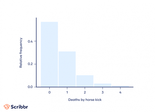
For example, Ladislaus Bortkiewicz calculated the deaths of soldiers by horse kicks in the Prussian Army using Poisson Distribution in the late 1800s. He analyzed two decades of data from up to 10 army corps, equivalent to two centuries of observations for one army corps.
Figure 1: Poisson Distribution for deaths by horse kick by Ladislaus Bortkiewicz. Source: Scribbr
According to his observation, an average of 0.61 soldiers died every year. However, the deaths were random, for example, in one year four soldiers died and for most years no deaths were caused by horses. Figure 1 shows the probability mass function graph. In Poisson Distribution terms,
- Death caused by a horse kick is an ‘event’
- Mean per time interval, represented by λ, is 0.61
- The number of deaths by horse kick in a specific year is k.
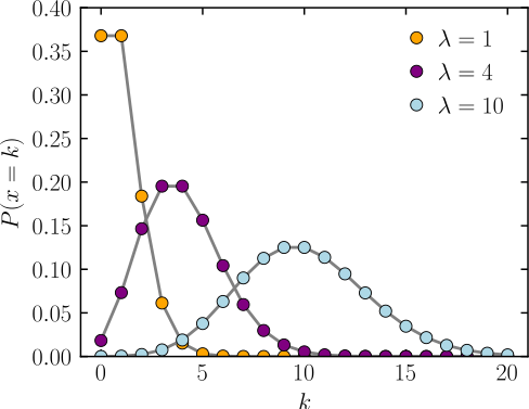
Figure 2 is the probability mass function of the Poisson distribution and shows the probability (y-axis) of a number of events (x-axis) occurring in one interval with different rate parameters. You can see the most likely number of event occurrences for a graph is equivalent to its rate parameter (λ) as it is the expected number of events in one interval when it is an integer. When it is not an integer, the number of events with the highest probability would be nearest to λ. The Lamda, λ, also represents the mean and variance of the distribution.
4. Features and Properties
Some properties of Poisson distribution are:
1. As seen in figure 2, if a quantity is Poisson Distributed with rate parameter, λ, its average value is λ.
2. Variance of the distribution is also λ, implying when λ increases the width of the distribution goes as square root lambda √λ.
3. A converse in Raikov’s theorem says that if the sum of two independent random variables is Poisson distributed, then so are each of those two independent random variables Poisson distributed.
Consider the example of radioactive decay for long-lived isotopes, in a radioactive sample containing a large number of nuclei, each of which has a tiny probability of decaying during some time interval, T. Let’s say the rate of decay is 0.31 decay/second and is monitored for 10 seconds. That gives us the λ1 0.31 * 10 = 3.1 which means the probability equals,
Consider another example where λ2 is 2.7, the probability is
Therefore, If we look at the total number k = k1 + k2 of a radioactive decay in a time T, the result is also a Poisson distribution with λ = λ1 + λ2 -> λ = 3.1 + 2.7 = 5.8 : P(k, λ1 + λ2 )
If we have two independent Poisson-distributed variables, their sum is Poisson distributed too.
4. The skewness is measured by 1/√λ
5. Excess kurtosis is measured by 1/λ. See the difference between excess kurtosis and kurtosis here. In a nutshell, excess kurtosis compares the kurtosis of the distribution with the kurtosis of a normal distribution and can therefore tell you if an (extreme) event is more or less likely in this case than if the distribution followed a normal distribution.
6. Poisson Limit Theorem states that Poisson distribution may be used as an approximation to the binomial distribution, under certain conditions. When the value of n (number of trials) in a binomial distribution is large and the value of p (probability of success) is very small, the binomial distribution can be approximated by a Poisson distribution i.e., n -> ∞ and λ = np, rate parameter, λ is defined as the number of trials, n, in binomial distribution multiplied by the probability of success, p.
7. A Poisson distribution with a high mean λ > 20 can be approximated as a normal distribution. However, as normal distribution is a continuous probability distribution, a continuity correction is necessary. It would exceed the scope to discuss in detail here what this correction is. In short, it adds or substracts 0.5 to the value in question to increase the accuracy of the estimation when using a continuous probability approach for something that has discrete probabilities. For example, a factory with 45 accidents per year follows a Poisson distribution. A normal approximation would suggest that the probability of more than 50 accidents can be computed as follows:
Mean = λ = μ =45
Standard deviation = ∂ = √λ = 6.71 P(X>50.5) -> after continuity correction =
using Z score table, see more here.
5. Poisson Distribution in Python
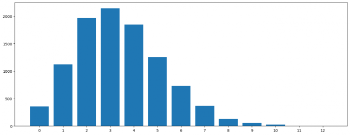
The following example generates random data on the number of duststorms in the city of Multan. The lambda is set at 3.4 storms per year and the data is monitored for 10,000 years.
#import libraries

from scipy.stats import poisson ## to calculate the passion distribution
import numpy as np ## to prepare the data
import pandas as pd ## to prepare the data
import matplotlib.pyplot as plt ## to create plots
#Random Example: Modeling the frequency of the number of duststorms in Multan, Pakistan

#creating data for 10000 years using scipy.stat.poisson library
#Rate lamda = 3.4 duststorm in Multan every year

d_rvs = pd.Series(poisson.rvs(3.4, size=10000, random_state=2)) #random_state so we can reproduce it #turning into panda series
d_rvs[:20] # first 20 entry, so the first 20 years, with the number of storms on the right
d_rvs.mean() # mean of 10000 values is 3.3879, approximately what we set as the average number of duststorm per year.
Outcome: 3.3879
#showing the frequency of years against the number of storms per year and sorting it by index.
data = d_rvs.value_counts().sort_index().to_dict() #storing in a dictionary
data
## You can see that most years have 2-4 storms which is also represented in the calculated average and our lambda.
Outcome:
0: 357,
1: 1122,
2: 1971,
3: 2144,
4: 1847,
5: 1253,
6: 731,
7: 368,
8: 126,
9: 54,
10: 24,
11: 2,
12: 1
fig, ax = plt.subplots(figsize=(16, 6))
ax.bar(range(len(data)), list(data.values()), align='center')
plt.xticks(range(len(data)), list(data.keys()))
plt.show()
The resulting pmf confirms that the closest integer value to lamba i.e., 3 has the most number of years out of 10,000 meaning most years will have 3 duststorms. You can also see that the data is slightly skewed to the right since there is a larger variance to the right than to the left. Looking at the distribution, it looks fairly normally distributed. However, the low lambda does not allow to use the Poisson distribution as an approximation for a normal distribution. Most probably, the large dataset allows us to see it as a normal distribution, since most distributions converge to a normal distribution with increasing sample size.
6. References
- Brownlee, Jason: "A Gentle Introduction to Probability Distributions", 14.11.2019. Retrieved from: https://machinelearningmastery.com/what-are-probability-distributions/#:~:text=A%20probability%20distribution%20is%20a,properties%20that%20can%20be%20measured, last checked: 21.05.2023
- Koehrsen, Will: " The Poisson Process and Poisson Distribution Explained (With Meteors!), 28.10.2022. Retrieved from: https://builtin.com/data-science/poisson-process, last checked: 21.05.2023
- Papoulis, Athanasios; Pillai, S. Unnikrishna: "Probability, Random Variables, and Stochastic Processes" (4th ed.).
- Raikov, Dmitry (1937): "On the decomposition of Poisson laws". Comptes Rendus de l'Académie des Sciences de l'URSS. 14: 9–11.
The author of this entry is XX. Edited by Milan Maushart


