Mathematics of the t-Test
In short: The (Student’s) t-distributions ares a family of continuous distributions. The distribution describes how the means of small samples of a normal distribution are distributed around the distributions true mean. T-tests can be used to investigate whether there is a significant difference between two groups regarding a mean value (two-sample t-test) or the mean in one group compared to a fixed value (one-sample t-test).
This entry focuses on the mathematics behind T-tests and covers one-sample t-tests and two-sample t-tests, including independent samples and paired samples. For more information on the t-test and other comparable approaches, please refer to the entry on Simple Statistical Tests. For more information on t-testing in R, please refer to this entry.
Contents
t-Distribution
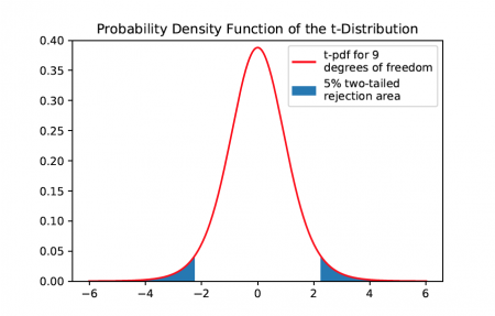
The (Student’s) t-distributions ares a family of continuous distributions. The distribution describes how the means of small samples of a normal distribution are distributed around the distributions true mean. The locations x of the means of samples with size n and ν = n−1 degrees of freedom are distributed according to the following probability distribution function:
The gamma function:
For integer values:
The t-distribution is symmetric and approximates the normal distribution for large sample sizes.
t-test
To compare the mean of a distribution with another distributions mean or an arbitrary value μ, a t-test can be used. Depending on the kind of t-test to be conducted, a different t-statistic has to be used. The t-statistic is a random variable which is distributed according to the t-distribution, from which rejection intervals can be constructed, to be used for hypothesis testing.
One-sample t-test
When trying to determine whether the mean of a sample of n data points with values xi deviates significantly from a specified value μ, a one-sample t-test can be used. For a sample drawn from a standard normal distribution with mean μ, the t-statistic t can be constructed as a random variable in the following way:
The numerator of this fraction is given as the difference between x, the measured mean of the sample, and the theorized mean value μ.
The denominator is calculated as the fraction of the samples standard deviation σ and the square-root of the samples size n. The samples standard deviation is calculated as follows:
The t statistic is distributed according to a students t distribution. This can be used to construct confidence intervals for one or two-tailed hypothesis tests.
Two-sample t-test
When wanting to find out whether the means of two samples of a distribution are deviating significantly. If the two samples are independent from each other, an independent two-sample t-test has to be used. If the samples are dependent, which means that the values being tested stem from the same samples or that the two samples are paired, a paired t-test can be used.
Independent Samples
For independent samples with similar variances (a maximum ratio of 2), the t-statistic is calculated in the following way:
with the estimated pooled standard deviation
In accordance with the One-sample t-test, the sample sizes, means and standard deviations of the samples 1 and 2 are denoted by n1/2, x1/2 and σx1/2 respectively. The degrees of freedom which are required for conducting the hypothesis testing is given as ν = n1 + n2 − 2. For samples with unequal variances, meaning that one sample variance is more than twice as big as the other, Welch’s t-test has to be used, leading to a different t-statistic t and different degrees of freedom ν:
An approximation for the degrees of freedom can be calculated using the Welch-Satterthwaite equation:
It can be easily shown, that the t-statistic simplifies for equal sample sizes:
Paired Samples
When testing whether the means of two paired samples are differing significantly, the t-statistic consists of variables that differ from the ones used in previous tests:
Instead of the independent means and standard deviations of the samples, new variables are used, that depend on the differences between the variable pairs. xd is given as the average of the differences of the sample pairs and σD denotes the corresponding standard deviation. The value of μ0 is set to zero to test whether the mean of the differences takes on a significant value.
The authors of this entry is Moritz Wohlstein.


