K-Means Algorithm in Python
THIS ARTICLE IS STILL IN EDITING MODE
Contents
Introduction
K-means is one of the simplest unsupervised learning algorithms that solve the clustering problem, in other words, classify a given dataset on a certain number of clusters (assume k clusters) fixed a priori.
Theoretical aspect
The main idea is to define k centroids, one for each cluster. These centroids should be placed in a cunning way because different location causes different result. Therefore, the better choice is to place them as much as possible far away from each other. The next step is to take each point belonging to a given data set and associate it to the nearest centroid. When no point is pending, the first step is completed and an early group is done. At this point, it is needed to recalculate k new centroids as centers of the clusters resulting from the previous step. After that a new binding has to be done between the same data points and the nearest new centroid. A loop has been generated. As a result of this loop the centroids change their location step by step until no more changes are done, so centroids do not move any more.
For a given dataset X containing n multidimensional data points and the number of categories k to be divided, the Euclidean distance is selected as the similarity index and the clustering aims to minimize the sum of the squares of the various types:
where k - cluster centers, n - number of data points, uk - the kth center, and xi the ith point in the data set.
The algorithm consists of the following steps:
1. Place k points in the space represented by the objects that are being clustered. These points are considered as initial group centroids.
2. Assign each object to the group that has the closest centroid.
3. When all objects have been assigned, recalculate the positions of the k centroids.
4. Repeat Step 2 and 3 until the centroids stop moving.
Python Example
RFM analysis
Recency, frequency and monetary (RFM) analysis is a powerful and recognized technique in database marketing. It is widely used to rank the customers based on their prior purchasing history.
1. Recency: When was the last time the customer made a purchase?
2. Frequency: How many times did the customer purchase?
3. Monetary: How much money did the customer spend?
import pandas as pd
import numpy as np
import matplotlib.pyplot as plt
import seaborn as sns
import datetime as dt

from sklearn.cluster import KMeans
from sklearn.neighbors import NearestNeighbors

from sklearn import metrics

#loading dataset (we use online retail dataset)
df = pd.read_excel(r"filepath\online_retail.xlsx")
df
| Column1 | CustomerID | OrderID | Date | Revenue | date_format | YEAR | month | |
|---|---|---|---|---|---|---|---|---|
| 0 | 111382 | 13930366 | 43771330 | 20191023 | 5834 | 2019-10-23 | 2019 | 10 |
| 1 | 111385 | 11545838 | 43723657 | 20191023 | 5834 | 2019-10-23 | 2019 | 10 |
Recency
# last date available in our dataset
df["date_format"].max() # Out: Timestamp('2020-04-19 00:00:00')

# setting max time as now to calculate time differences
now = dt.date(2020,4,19)
# group by customer by last date they purchased

df_recency = df.groupby(["CustomerID"] , as_index = False)["date_format"].max()
df_recency.columns = ["CustomerID" , "LastPurchaseDate"]
df_recency["LastPurchaseDate"] = pd.DatetimeIndex(df_recency.LastPurchaseDate).date
df_recency.head()
| CustomerID | LastPurchaseDate | |
|---|---|---|
| 0 | 465132 | 2019-11-30 |
| 1 | 465164 | 2020-02-28 |
| 2 | 465198 | 2020-04-13 |
| 3 | 465204 | 2019-11-03 |
| 4 | 465211 | 2020-01-22 |
# calculate how often the customers are buying in the last few days
df_recency['Recency'] = df_recency.LastPurchaseDate.apply(lambda x : (now - x).days)

# dropping LastPurchase Date
df_recency.drop(columns=['LastPurchaseDate'],inplace=True)

# checking recencyFrequency
df_recency.head()
| CustomerID | Recency | |
|---|---|---|
| 0 | 465132 | 141 |
| 1 | 465164 | 51 |
| 2 | 465198 | 6 |
| 3 | 465204 | 168 |
| 4 | 465211 | 88 |
Frequency
frequency_df = df.groupby("CustomerID",as_index = False)["OrderID"].count()
frequency_df = frequency_df.sort_values(by = "OrderID" , ascending=False)
frequency_df = frequency_df.rename(columns={"OrderID" :"Frequency"})
frequency_df.head()
| CustomerID | Frequency | |
|---|---|---|
| 1525 | 502561 | 231 |
| 66329 | 5556237 | 180 |
| 136996 | 11826511 | 159 |
| 137116 | 11836775 | 153 |
| 164161 | 14188909 | 143 |
Monetary
# check summed up spends of customers

monetary_df = df.groupby('CustomerID',as_index=False)["Revenue"].sum()
monetary_df.columns = ['CustomerID','Monetary']
monetary_df.head()
| CustomerID | Monetary | |
|---|---|---|
| 0 | 465132 | 7302 |
| 1 | 465164 | 578 |
| 2 | 465198 | 5688 |
| 3 | 465204 | 1464 |
| 4 | 465211 | 4760 |
# merging these three features
rf = df_recency.merge(frequency_df,left_on='CustomerID',right_on='CustomerID')

# combining with monetary values
rfm = rf.merge(monetary_df,left_on='CustomerID',right_on='CustomerID')

rfm.set_index('CustomerID',inplace=True)

# saving to file
rfm.to_csv('rfm.csv', index=False)
#rf_new = rfm.sort_values(by = "Frequency" , ascending = False)

# checking the dataframe
rfm.head()
| CustomerID | Recency | Frequency | Monetary |
|---|---|---|---|
| 465132 | 141 | 1 | 7302 |
| 465164 | 51 | 1 | 578 |
| 465198 | 6 | 1 | 5688 |
| 465204 | 168 | 1 | 1464 |
| 465211 | 88 | 1 | 4760 |
Segmentation and Evaluation
In the literature several approaches have been proposed to determine the number of clusters for k-mean clustering algorithm, for instance: i) Rule of thumb; ii) Elbow method; iii) Information Criterion Approach; iv) Information Theoretic Approach; v) Silhouette method and vi) Cross-validation.
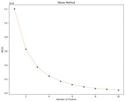
In this case we will use Elbow method to determine the number of clusters. The basic idea of the elbow rule is to use a squareed distance between the sample points in each cluster and the centroid of the cluster to give a series of K values. The sum of squared errors (SSE) is used as a performance indicator. The method iterates over the K-value and calculates the SSE.
# creating a copy of the dataframe
rfm_segmentation = rfm.copy()

# find the proper number of clusters
fig,ax = plt.subplots(figsize=(10,8))
wcss = []
for i in range(1,11):
  kmeans = KMeans(n_clusters = i, init = 'k-means++', max_iter = 300, n_init = 10, random_state = 0)
  kmeans.fit(rfm_segmentation)
  wcss.append(kmeans.inertia_)
plt.plot(range(1,11), wcss, 'o')
plt.plot(range(1 , 11) , wcss , '-' , alpha = 0.5)
plt.title('Elbow Method')
plt.xlabel('Number of Clusters')
plt.ylabel('WCSS')
plt.savefig('Elbow_Method.png')
plt.show()
The graph shows, that the curve changes its behaviour from steep to moderate slope at the point of 4 clusters, therefore, we will choose 3 as the proper number of clusters for k-means segmentation. This will be included in the model as a parameter.
# instantiating the model

kmeans = KMeans(n_clusters = 3, init = 'k-means++', max_iter = 300, n_init = 10, random_state = 0)
y_kmeans = kmeans.fit_predict(rfm_segmentation)

# creating a column for the cluster

rfm_segmentation['Cluster'] = kmeans.labels_

# checking the column
rfm_segmentation[rfm_segmentation.Cluster == 0].head()
| CustomerID | Recency | Frequency | Monetary | Cluster |
|---|---|---|---|---|
| 465132 | 141 | 1 | 7302 | 0 |
| 465164 | 51 | 1 | 578 | 0 |
| 465198 | 6 | 1 | 5688 | 0 |
| 465204 | 168 | 1 | 1464 | 0 |
| 465211 | 88 | 1 | 4760 | 0 |
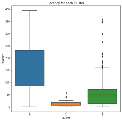
As we applied clustering, we are now able to analyze Recency, Frequency and Monetary values for each group.
Recency rate analysis
fig, ax = plt.subplots(figsize=(8,8))
plt.title('Recency for each Cluster')
sns.boxplot(rfm_segmentation.Cluster,rfm_segmentation.Recency)
plt.savefig("recency_clusters.png")
Cluster 0 has high recency rate, respectively, which means it has been the longest for any cluster when it comes to Last Purchase Date.
Cluster 1 and 2 have low recency rate, which is good. They can be our Gold and Silver Customers.
Frequency rate analysis
fig, ax = plt.subplots(figsize=(8,8))
plt.title('Frequency for each Cluster')
sns.boxplot(rfm_segmentation.Cluster,rfm_segmentation.Frequency);
plt.savefig('frequency_cluster.png')
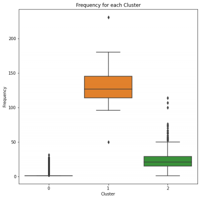
Cluster 0 has a low frequency rate, which means consumers in this cluster are not very frequent.
Clusters 1 and 2 have high frequency rates, which puts them even further in the race for Gold and Silver.
Monetary rate analysis
fig, ax = plt.subplots(figsize=(8,8))
plt.title('Monetary for each Cluster')
sns.boxplot(rfm_segmentation.Cluster,rfm_segmentation.Monetary);
plt.savefig('monetary_cluster.png')
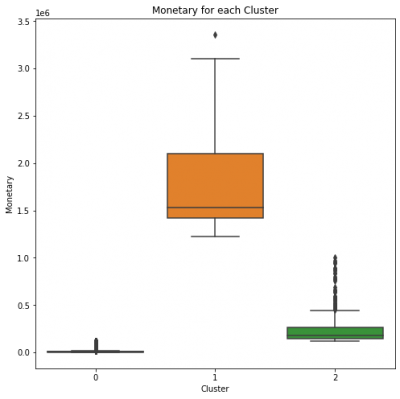
Cluster 0 has a small monetary rate, which could be referred to Bronze Customers.
Cluster 2 has a medium level monetary rate, which makes this Cluster to be Silver Customers.
Cluster 1 has the highest monetary rate, suggesting this Cluster to be Gold Customers.
Result
We may conclude the following results, based on analyses:
- Gold Customers are in Cluster 1.
- Silver Customers are in Cluster 2.
- Bronze Customers are in Cluster 0.
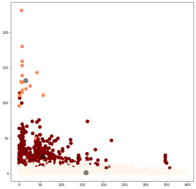
Visualization
# getting the values
X = rfm_segmentation.iloc[:, [0,1,2]].values

# 2d plot
fig, ax = plt.subplots(figsize=(10,10))
plt.scatter(X[:, 0], X[:, 1], c=y_kmeans, s=100, cmap='OrRd')

centers = kmeans.cluster_centers_
plt.scatter(centers[:, 0], centers[:, 1], c='black', s=200, alpha=0.5)
# checking number of clients per cluster
rfm_segmentation.Cluster.value_counts()
| 0 | 179083 |
| 2 | 581 |
| 1 | 16 |
Strenghts and Drawbacks of k-means Algorithm
Strenghts:
1. Simple.
2. Fast for low dimensional data.
3. It can find pure sub clusters, if large number of clusters is specified.
4. With a large number of variables, k-Means may be viewed as computationally faster than hierarchical clustering.
5. K-Means is expected to produce tighter clusters than hierarchical clustering.
Drawbacks:
1. Sensitive to the selection of initial cluster center.
2. There is no rule for the decision of value of k and sensitive to initial value , for different initial value there will be different result.
3. This algorithm is easy to be effected by abnormal points.
4. It may contain dead unit problem.
References
2. https://www.mdpi.com/2571-8800/2/2/16
The author of this entry is Faezeh Moradi. Edited by Evgeniya Zakharova.

