Decision Trees in Python

THIS ARTICLE IS STILL IN EDITING MODE

In short: Decision tree learning is a supervised machine learning method that is both used for classification and regression problems. It is a very powerful method that is also easy to interpret and understand. However, decision trees can easily encounter overfitfing and therefore not generalize well. Often, methods such as pruning have to be applied.

Motivation

Decision tree learning falls into the category of supervised machine learning algorithms. The final predictive model is referred to as decision tree. Decision trees can be used for both regression (regression trees) and classification tasks (classification trees). Thus, they can be used whenever the dataset that contains features and a target variable. For instance, consider the following dataset from Mitchell (1997) (table 1). Outlook, temperature, humidity, and wind are the features, and the target variable is whether we should play tennis or not. Can we find a pattern in the data that allows us to determine this on a given day?

Table 1. Training examples for the target concept PlayTennis

Day	Outlook	Temperature	Humidity	Wind	PlayTennis
Dl	Sunny	Hot	High	Weak	No
D2	Sunny	Hot	High	Strong	No
D3	Overcast	Hot	High	Weak	Yes
D4	Rain	Mild	High	Weak	Yes
D5	Rain	Cool	Normal	Weak	Yes
D6	Rain	Cool	Normal	Strong	No
D7	Overcast	Cool	Normal	Strong	Yes
D8	Sunny	Mild	High	Weak	No
D9	Sunny	Cool	Normal	Weak	Yes
D10	Rain	Mild	Normal	Weak	Yes
D11	Sunny	Mild	Normal	Strong	Yes
D12	Overcast	Mild	High	Strong	Yes
D13	Overcast	Hot	Normal	Weak	Yes
D14	Rain	Mild	High	Strong	No

What the Method does

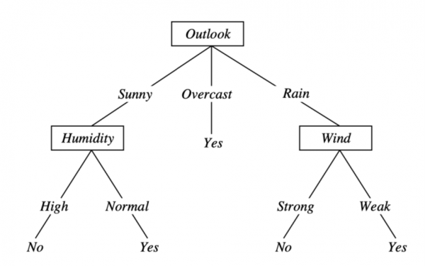
A decision tree breaks down this complex decision of whether one should or should not play tennis into a set of logical rules using disjunctions (OR) and conjunctions (AND). A decision tree for this dataset may look as follows: I will play tennis whenever…

- the outlook today is overcast; - OR if the outlook is sunny AND the humidity is normal; - OR the outlook is rain AND the wind is weak.

The algorithm first selects the most informative feature for the root node of the tree and splits the data into subsets that correspond to the branches of the feature. There are different metrics on how to calculate the most informative feature (e.g., entropy or Gini impurity for classification, variance for regression), though generally, they all measure the homogeneity of the target variable in the respective subset of the data and choose the feature with the highest homogeneity.

In our example, outlook was selected as the most informative feature and the subsets would be all the data where outlook is sunny, overcast or rain. The algorithm then repeats the same procedure on all the subsets that were created. It stops once the target variable in a subset is homogeneous, meaning that all the examples belong to the same class.

Interpretability

One big advantage of decision trees is that they are considered to be human interpretable. Compared to other models, such as neural networks, decision trees are white box models. Any prediction of the tree can be explained by Boolean logic. On top of that, we can also visualize the final model and arrive at the same conclusion as the decision tree by following the branches of the tree. The following picture (Figure 1) shows the same logical rules that were previously mentioned.

Simple Regression Tree Model in Python

In this example, we are going to use the car price prediction dataset from Kaggle. The goal is to predict the price of a car based on certain properties of cars, such as car length, cylinder size, etc.

First, we have to import the libraries and modules that we will use for this demonstration.

import pandas as pd
import numpy as np 
from sklearn import tree
from sklearn.model_selection import train_test_split
from sklearn.metrics import mean_squared_error, r2_score

Note that this dataset is a toy dataset, meaning that luckily for us, not a lot of data-cleaning and preprocessing will have to be done. The accuracy of our model could potentially be improved by including more preprocessing steps or model simplification. However, the purpose of this example is not necessarily how to achieve the highest accuracy (then we would use more sophisticated models, such as random forest regression). Instead, the goal is to showcase how one could employ a simple decision tree model. We are now going to import our data using pandas.

df = pd.read_csv('CarPrice_Assignment.csv')
df.columns

Index(['car_ID', 'symboling', 'CarName', 'fueltype', 'aspiration',

      'doornumber', 'carbody', 'drivewheel', 'enginelocation', 'wheelbase',
      'carlength', 'carwidth', 'carheight', 'curbweight', 'enginetype',
      'cylindernumber', 'enginesize', 'fuelsystem', 'boreratio', 'stroke',
      'compressionratio', 'horsepower', 'peakrpm', 'citympg', 'highwaympg',
      'price'],
     dtype='object')

We are going to remove the car_ID column, as it is basically the same as the index. Let us do some modifications of the CarName column, in order to display only the car`s brand avoiding typos.

# Drop useless column
df = df.drop(columns='car_ID',axis=1)

def car_brand(car_name):
    # This function takes an entry of the 'carName' column and splits the words into a list. 
    # The first word will be the car brand, which is then returned in lowercase. 
    car_brand = car_name.split(" ")[0].lower()
    return car_brand

# We apply the car_brand function to the 'CarBrand' column
df['CarBrand']=df['CarName'].apply(car_brand)

# Drop the old 'CarName' column from the dataframe
df.drop(columns='CarName',axis=1,inplace=True)

# Fixing some typos 
df.loc[df['CarBrand']=='vokswagen','CarBrand']='vw'
df.loc[df['CarBrand']=='volkswagen','CarBrand']='vw'
df.loc[df['CarBrand']=='porcshce','CarBrand']='porsche'
df.loc[df['CarBrand']=='maxda','CarBrand']='mazda'
df.loc[df['CarBrand']=='toyouta','CarBrand']='toyota'
df.columns

Even though categorical data works for decision trees, the Scikit-Learn implementation does not support this kind of data. Since our categorical columns do not contain ordinal data, we have to one-hot encode the categorical columns. We could also standardize the numeric columns (except our target variable) to have a mean 0 and a standard deviation of 1. However, decision trees do not require this assuption and can handle unstandardized data.

# Collect the categoric and numeric columns in a list
categoric = df.select_dtypes(include=object).columns.to_list()
# One-hot encode the categoric columns
df_cat = pd.get_dummies(df[categoric], dtype=float)
# First drop the old categoric columns and then concat the new categoric columns onto the original dataframe
df = df.drop(columns=categoric)
df = pd.concat([df, df_cat], axis= 1)

We now split the data into training and test set and fit our decision tree model. We then simply have to initialize the DecisionTreeRegressor (DecisionTreeClassifier for classification) class. We use a random state for reproducibility.

# Convert data into features X and labels y in a numpy array
X = np.asarray(df.drop(columns='price', axis=1))
y = np.asarray(df['price'])

# Split the data into train and test sets
X_train, X_test, y_train, y_test = train_test_split(X, y, test_size=0.33, random_state=0)

# Set the minimum number of samples in each leaf to 5 to pre-prune the tree
reg_tree = tree.DecisionTreeRegressor(random_state=0)

# Fit the model
reg_tree.fit(X_train, y_train)

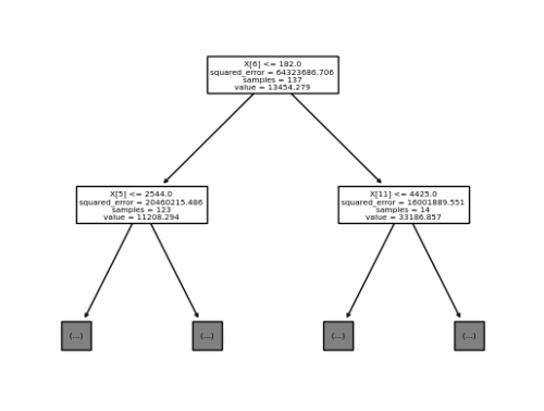
After the DecisionTreeRegressor instance was fitted, we can plot the tree as follows:

from matplotlib import pyplot as plt

tree.plot_tree(reg_tree, max_depth=1)
plt.show() # Figure 2

Further explanation and other parameters of the method plot_tree can be found here.

Lastly, we calculate the root mean squared error (RSME) for our train and test predictions and also calculate the coefficient of determination to evaluate how well the model fits the data.

y_pred_train = reg_tree.predict(X_train)

# Train RMSE 
RMSE_train = np.sqrt(mean_squared_error(y_train, y_pred_train))
print("RMSE for Training Data: ", RMSE_train) # Out: 291.4381969264448

# Train R_squared
R_squared_train = r2_score(y_train, y_pred_train)
print("Training R_squared for Decision Tree Regression Model: ", R_squared_train) # Out: 0.9986795498364933

We see that our model can almost perfectly explain the training data. The next step will be to check the measurements for the test data:

y_pred_test = reg_tree.predict(X_test)

# Test RMSE 
RMSE_test = np.sqrt(mean_squared_error(y_test, y_pred_test))
print("RMSE for Testing Data: ", RMSE_test)

# Test R_squared:
R_squared_test= r2_score(y_test, y_pred_test) # Out: 2839.9804482339855
print("Testing R_squared for Decision Tree Regression Model: ", R_squared_test) # Out: 0.8692375508177494

The results show that Test RMSE is much more than for the training data, in turn, Test R_squared is less. We may suggest that it is overfitting. This is an disadvantage of decision trees. A decision tree can potentially split the data until each subset is completely homogeneous, which basically means that our tree has memorized the data and won’t extrapolate to unseen data.

Pre- and Post-Pruning

In order to counteract the problem of overfitting, we can prune our decision tree. Pruning the tree will reduce the depth of the tree which hinders it to perfectly match all training examples.

Pre-Pruning

One way to prune the tree is to set a limit on the its depth beforehand. This method is referred to as pre-pruning or early stopping. However, this can be a bit tricky because we do not know how to set the parameters in advance. In order to implement this, the max_depth parameter can be used, when initializing the tree. Alternatively, we can also require the tree to have a certain number of examples in the leaf nodes through the min_samples_leaf parameter. Let us see how well our model performs on the test set, using a pre-pruning method.

# Set the minimum number of samples in each leaf to 5 to pre-prune the tree
reg_tree = tree.DecisionTreeRegressor(random_state=0, min_samples_leaf=4)

# Train the model 
reg_tree.fit(X_train, y_train)

# Collect the predictions of the train and test data
y_pred_train = reg_tree.predict(X_train)
y_pred_test = reg_tree.predict(X_test)

# Train RMSE 
RMSE_train = np.sqrt(mean_squared_error(y_train, y_pred_train))
print("RMSE for Training Data: ", RMSE_train) # Out: 1464.1947006424898

# Test RMSE
RMSE_test = np.sqrt(mean_squared_error(y_test, y_pred_test))
print("RMSE for Testing Data: ", RMSE_test) # Out: 2541.4558310183947

# Train R_squared:
R_squared_train = r2_score(y_train, y_pred_train)
print("Training R_squared for Decision Tree Regression Model: ", R_squared_train) # Out: 0.9666706584900479

# Test R_squared:
R_squared_test = r2_score(y_test, y_pred_test)
print("Testing R_squared for Decision Tree Regression Model: ", R_squared_test) # Out: 0.8952829308308532

We can see that the model accuracy on the training data has decreased. However, we can generalize better on unseen data than before without any pruning.

Post-Pruning

Post-pruning is a method where first we let the decision tree overfit the data. Then, using a validation set, we prune the tree and remove the nodes, where deleting them would increase the validation performance the most. It is a bit more complex mathematically. An example can be found here.

Strength & Weaknesses of Decision Trees

Weaknesses

• Overfitting is an often issue. Therefore, pruning methods need to be applied.
• Decision trees are sensitive to noise. More sophisticated models such as random forests can help to overcome this.
• If the dataset is unbalanced, then decision trees can create a biased model.

Strengths

• As it was previously pointed out, decision trees are white box models. As long as they are not too large, they can be visualized and interpreted easily by humans.
• They are relatively simple to use.
• Can be used for both categorical and numerical data.
• Require little data-preprocessing, e.g., decision trees can handle unstandardized data and missing values.

References

1. 1.10. Decision Trees. (n.d.). Scikit-learn. https://scikit-learn.org/stable/modules/tree.html

2. Post pruning decision trees with cost complexity pruning. (n.d.). Scikit-learn. https://scikit-learn.org/stable/auto_examples/tree/plot_cost_complexity_pruning.html

3. Mitchell, T. (1997). Machine Learning.

4. Shalev‐Shwartz, S., & Ben-David, S. (2014). Understanding machine learning. https://doi.org/10.1017/cbo9781107298019

The author of this entry is Moritz Burmester. Edited by Evgeniya Zakharova.