Simple Statistical Tests
| Method categorization | ||
|---|---|---|
| Quantitative | Qualitative | |
| Inductive | Deductive | |
| Individual | System | Global |
| Past | Present | Future |
In short: Simple statistical tests encapsule an array of simple statistical tests that are all built on probability, and no other validation criteria.
Contents
Background
Simple testing statistics provide the baseline for advanced statistical thinking. While they are not so much used today within empirical analysis, simple tests are the foundation of modern statistics. The student t-test which originated around 100 years ago provided the crucial link from the more inductive thinking of Sir Francis Bacon towards the testing of hypotheses and the actual statistical testing of hypotheses. The formulation of the so-called null hypothesis is the first step within simple tests. Informed from theory this test calculates the probability whether the sample confirms the hypothesis or not. Null hypotheses are hence the assumptions we have about the world, and these assumptions can be confirmed or rejected.
Most relevant simple tests
one sample t-test

It allows for the comparison of a sample to a pre-defined reference value. It tells you whether the mean of your sample differs significantly from this value. For this purpose, the t-test gives you a p-value at the end. If the p-value is below 0.05, the sample differs significantly from the reference value.
Example: Do the packages of your favourite cookie brand always contain as many cookies as stated on the outside of the box? Collect some of the packages, weigh the cookies contained therein and calculate the mean weight. Now, you can compare this value to the weight that is stated on the box using a one sample t-test.
two sample t-test

It allows a comparison of two different datasets or samples within an experiment. It tells you if the means of the two datasets differ significantly. If the p-value is below 0,05, the two samples differ significantly.
Example: The classic example would be to grow several plants and to add fertiliser to half of them. We can now compare the gross of the plants between the control samples without fertiliser and the samples that had fertiliser added.
Plants with fertiliser (cm): 7.44 6.35 8.52 11.40 10.48 11.23 8.30 9.33 9.55 10.40 8.36 9.69 7.66 8.87 12.89 10.54 6.72 8.83 8.57 7.75
Plants without fertiliser (cm): 6.07 9.55 5.72 6.84 7.63 5.59 6.21 3.05 4.32 8.27 6.13 7.92 4.08 7.33 9.91 8.35 7.26 6.08 5.81 8.46
The result of the two-sample t-test is a p-value of 7.468e-05, which is close to zero and definitely below 0,05. Hence, the samples differ significantly and the fertilizer is likely to have an effect.
Paired t-test

It allows for a comparison of a sample before and after an intervention. Within such an experimental setup specific individuals are compared before and after an event. If the sample changes significantly, comparing start and end state, you will receive again a p-value below 0,05.
Example: Your level of concentration in the morning before and after having a cup of coffee.
Wilcoxon Test

It is also a paired test (see paired t-test), but you can use it if your sample is (exceptionally) NOT normally distributed, e.g. if one sample is skewed or if there are large gaps in the data. Regardless of these issues, the test will tell you if the means of two samples differ significantly (i.e. p-value below 0,05) by using ranks.
Example: Imagine you have a sample where half of your people are professional basketball players then the real size of people would not make sense. Therefore, as a robust measure in modern statistics rank tests were introduced.
Chi-square Test of Stochastic Independence
The Chi Square test works for data that is only categorical. If you observe an event and measure two variables, you can use the Chi Square test to check if one variable influences the other one or if they occur independently from each other.
Example: Do the children of parents with an academic degree visit more often a university?
The H0 hypothesis would be: The variables are independent from each other.
The H1 hypotheses would be: The variables influence each other. For example because children from better educated families have higher chances to achieve good results in school.
For this example, the chi-quare test yields a p-value of 2.439e-07, which is close to zero. We can reject the null hypothesis H0 and assume that, based on our sample, the education of parents has an influence on the education of their children.
f-test


The test allows you to compare the variances of two samples. If the p-value is lower than 0,05, the variances differ significantly.
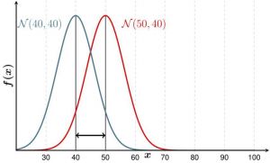
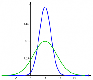
Example: If you examine players in a basketball and a hockey team, you would expect their heights to be different on average. But maybe the variance is not. Consider figure no. 1, where the mean is different, but the variance the same - this could be the case for your hockey and basketball team. In contrast, the height could be distributed as shown in figure no. 2. The f-test then would probably yield a p-value below 0,05.
Strengths & Challenges
(more to be added soon)
Requirements & Boundary Conditions
t-test
- The data of the sample(s) has to be normally distributed
- Dependend on the kind of t-test applied, the parent populations of the samples need to have the same variance (1)
Wilcoxon Test
Chi-square Test of Stochastical Independence
f-test
- The data of the samples has to be normally distributed
Normativity
Simple tests are not abundantly applied these days in scientific research, and often seem outdated. Much of the scientific designs and available datasets are more complicated, and many branches of sciences established more complex designs and a more nuanced view of the world. Consequently, simple tests grew kind of out of fashion. However, simple tests are not only robust, but sometimes still the most parsimonious approach. In addition, many simple tests are a basis for more complicated approaches, and initiated a deeper and more applied starting point for frequentist statistics. Simple tests are often the endpoint of many introductionary teachings on statistics, which is unfortunate. Overall, their lack in most of recent publications as well as wooden design frames of these approaches make these tests an undesirable starting point for many students, yet they are a vital stepping stone to more advanced models.
Outlook
Hopefully, one day school children will learn simple test, because they could, and the world would be all the better for it. If more people early on would learn about probability, and simple tests are a stepping stone on this long road, there would be an education deeper rooted in data and analysis, allowing for better choices and understanding of citizens.
Key Publications
- Student" William Sealy Gosset. 1908. The probable error of a mean. Biometrika 6 (1). 1–25.
- Cochran, William G. 1952. The Chi-square Test of Goodness of Fit. The Annals of Mathematical Statistics 23 (3). 315–345.
- Box, G. E. P. 1953. Non-Normality and Tests on Variances. Biometrika 40 (3/4). 318–335.
References
(1) Article on the "Student's t-test" on Wikipedia
Further information
The authors of this entry are Henrik von Wehrden and Carlo Krügermeier.

