Outlier Detection in Python
THIS ARTICLE IS STILL IN EDITING MODE
Outlier Detection in a nutshell: Outlier Detection includes methods identifying data points that deviate a lot from the rest of the data set.
Contents
Background
What is an outlier? An outlier is a data point that is significantly different from the other data points in a dataset. Its value is mostly unexpected and deviates a lot from the mean of the dataset. The task of outlier detection is to detect these points. However, one has to consider the context and the dataset when selecting a specific method for detecting outliers. Some examples of outliers include: 1. In a dataset of housing prices in a city, a data point representing a house that is significantly more or less expensive than the others could be an outlier. 2. In a dataset of exam scores for a class, a student who scores significantly higher or lower than the rest of the class could be an outlier. 3. In a dataset of consecutive GPS coordinates of sailing activities, coordinates with high deviation from the data points beforehand could be an outlier. Why is it important to detect outliers? Outlier detection is important because it helps to identify unusual or anomalous data points that may not fit with the rest of the data and therefore will have an impact on further analysis of the data. For instance, a linear regression model would be immensely affected by outliers and lose its ability to generalize well over the dataset.
Where is outlier detection located in the analysis process?' Outlier detection is typically a part of the data cleaning and exploration phase of the data analysis process. This is typically the first step in the process of analyzing a dataset, and it involves identifying and addressing any issues or problems with the data. Once the data has been cleaned and prepared, it can be analyzed using a variety of methods to draw conclusions, make predictions, or inform decisions
What are reasons for outliers? There are many possible reasons why outliers may occur in a dataset. Some common reasons include: 1. Measurement errors: Outliers can occur due to errors in the measurement process, such as incorrect readings or faulty equipment. 2. Data entry errors: Outliers can also occur due to errors in data entry, such as transposing numbers or mistyping data. 3. Natural variations: In some cases, outliers may occur naturally as a result of natural variations in the data. For example, extreme weather events or rare occurrences may result in data points that are significantly different from the rest of the data. 4. Fraud: Outliers can also occur as a result of fraudulent activity, such as attempts to manipulate data or hide certain transactions. 5. Sampling errors: In some cases, outliers may occur due to sampling errors, such as a sample that is not representative of the population being studied.
It is important to carefully consider the possible causes of outliers in a dataset, as this can help to identify and understand the underlying reasons for unusual data points. In some cases, it may be necessary to exclude outliers from analysis, while in other cases it may be important to include them to get a complete picture of the
Applying Methods in Python
n this section different methods for detecting outliers in datasets are presented using Python code. To demonstrate the methodology of different approaches, a dataset containing accelerometer data (captured during cycling activity) is used. More files like that can be found under the following Kaggle dataset: Kaggle Dataset.
In the first place, the dataset is loaded and limited to the first 10 seconds to make the visualizations of the outlier detection results better understandable.
data = pd.read_csv('Accelerometer_Data.csv', index_col=0)
data = data[data.time <= 10]
Visual Inspection
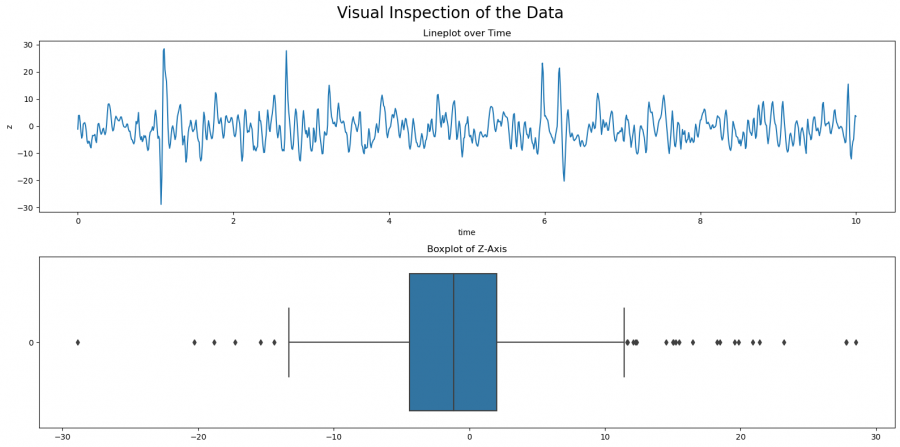
Already during the explorative data analysis with visualizations, you can make a first screening of the data for outliers using boxplots. For boxplots, the data is ordered from small to large to assess the distribution. It can then be seen how many data points lie outside the whiskers, i.e. deviate more than 1.5 from the inter-quartile range (IQR) from the mean value. The interquartile range represented by the box describes the range of 25-75% of the data distribution and the whiskers at the top and bottom the respective last 25%. Any data point outside the whiskers then is outliers. This methodology can be used as a basis for the subsequent quantile method to determine the corresponding thresholds/quantiles and to detect outliers from them.
fig, axs = plt.subplots(2, figsize=(16, 8))
fig.suptitle('Visual Inspection of the Data', size=20)
sns.lineplot(data=data, x='time', y='z', ax=axs[0])
axs[0].set(title='Lineplot over Time')
sns.boxplot(data['z'], orient='h', ax=axs[1])
axs[1].set(title='Boxplot of Z-Axis')
plt.tight_layout()
plt.show()
Figure 1: Visual Inspection of Outliers
We first create a plot with two subplots, one for the lineplot, and one for the boxplot. The line plot shows the development of the value z over time, and the boxplot shows the distribution with respect to the IQR of Z. You can see here already that there are some outliers. There are more outliers with larger than with smaller values. In the following, we will look at different approaches to detect outliers. Which method to use needs to be decided case by case, but you can compare the results in this article. In general, it is always advisable to try several approaches to fully understand your dataset.
Quantile Based
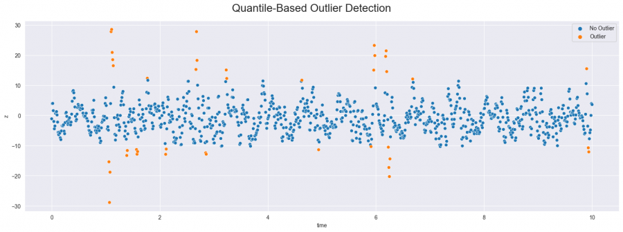
Quantile-based outlier detection is a fairly simple procedure in which points outside a certain quantile are considered outliers. For example, for thresholds 2 and 98 (as in the following code), all values that fall outside of these quantiles are marked as outliers. This means that data points at the top and bottom of the distribution are considered to be outliers. However, this approach runs the risk of incorrectly marking points as outliers since it does not take any further information about the distribution, like the standard deviation, into account.
# Set the quantiles and get the respective values
lower_q, upper_q = 0.02, 0.98## determine the qyartule thresholds.
lower_value = data['z'].quantile(lower_q)## apply the lower threshold to dataset.
upper_value = data['z'].quantile(upper_q)## apply the upper threshold to dataset.

# Plot the results
mask = (lower_value <= data.z) & (data.z <= upper_value)## create mask that differentiates between outlier and no outlier.
fig, ax = plt.subplots(figsize=(16, 6))## create a plot
fig.suptitle('Quantile-Based Outlier Detection', size=20) ## create title
sns.scatterplot(data=data, x='time', y='z', hue=np.where(mask, 'No Outlier', 'Outlier'), ax=ax) ## apply color to outlier/no outlier
plt.tight_layout() ##makes sure that all variables and axes are readable
plt.show()
Figure 2: Outliers detected with quantile-based method
Distribution Based
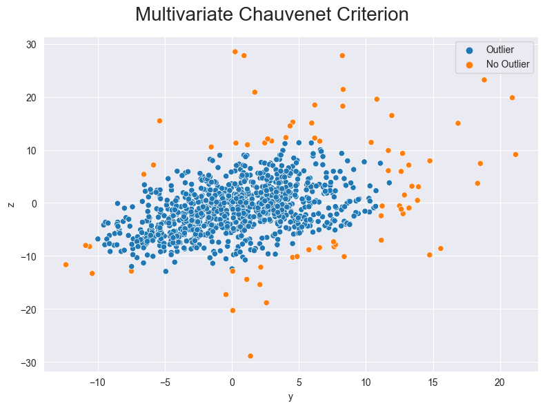
In distribution-based outlier detection, the assumption is made that data from a measurement are normally distributed. Based on the mean and standard deviation of the data, a probability results for each point of the recording that belongs to this normal distribution. Using the so-called Chauvenet criterion, a lower limit can be defined below which a point is marked as an outlier. If the Chauvenet criterion is set to 0.5, all points that belong to the normal distribution of the data with a probability of less than 0.5% are recognized as outliers. Depending on how high the criterion is set, the number of detected outliers changes accordingly (this is illustrated in figure 3). How high the optimal limit is, i.e. to which value the Chauvenet criterion must be set, depends on the further goal and is often only determined over time. This approach is closely related to the Z-score, which is a measure of the deviation of a point from the mean of a standardized normal distribution. The Chauvenet criterion can be applied to both univariate and multivariate data, offering the possibility to apply outlier detection either to single attributes or to a combination of attributes.
# Set the quantiles and get the respective values
lower_q, upper_q = 0.02, 0.98## determine the qyartule thresholds.
lower_value = data['z'].quantile(lower_q)## apply the lower threshold to dataset.
upper_value = data['z'].quantile(upper_q)## apply the upper threshold to dataset.

# Plot the results
def univariate_chauvenet(data_points: np.ndarray, criterion: float = None):
    # Calculate mean and std of the data
    mean = data_points.mean()
    std = data_points.std()

    # Calculate the criterion based on the number of points if not provided
    if criterion is None:
        criterion = 1.0/(2 * len(data_points)) ## criterion is set to 1 divided 2 times the length of the data set.

    # Calculate the absolute deviation and scale by std
    deviation = np.abs(data_points - mean) / std

    # Calculate the probabilities using erfc and return the mask. Erfc is the error function calculating the probability of a data point (not) being an outlier.
    # if the probability is lower than the criterion (so the likelihood that the data point is no outlier is smaller than the set criterion), it is an outlier.
    probabilities = special.erfc(deviation)
    return probabilities < criterion


fig, axs = plt.subplots(ncols=3, figsize=(16, 5))##create plot with three sub-plots
fig.suptitle('Univariate Chauvenet Criterion', size=20)
for i, c in enumerate([0.01, 0.005, 0.001]): ## creating a for loop to check for outliers for different criteria.
    mask = univariate_chauvenet(data_points=data['z'].values, criterion=c)## create mask as above
    sns.scatterplot(data=data, x='time', y='z', ax=axs[i],
                    hue=np.where(mask, 'Outlier', 'No Outlier'),
                    hue_order=['No Outlier', 'Outlier']) ##create scatter plots colored according to the mask.
    axs[i].set(title=f'Criterion = {c} with {sum(mask)} Outliers')
plt.tight_layout()
plt.show()
Figure 3: Outliers detected with the Chauvenet Criterion (univariate)
We can also show the z value and the y value in one graph with multivariate data.
def multivariate_chauvenet(data_points: np.ndarray, criterion: float = None) -> np.ndarray:
    # Calculate the mean and covariance matrix of data points
    mean = np.mean(data_points, axis=0)##determine mean for each column
    covariance = np.cov(data_points.T)## determine covariance between y and the value z. For this, the data points arrays need to be transposed.

    # Calculate criterion if not provided
    if criterion is None:
        criterion = 1 / (2 * len(data_points))

    def calculate_probability(x: np.ndarray) -> float:
        p = 1 / (2 * np.pi * np.linalg.det(covariance) ** 0.5) * \
            np.exp(-0.5 * np.matmul(np.matmul((x - mean), np.linalg.inv(covariance)), (x - mean)))
        return p ## calculate the probability of a data point X being in a multivariate normal distribution with a given probability density function

    # Calculate probabilities and return the mask
    probabilities = np.array([calculate_probability(x) for x in data_points])
    return probabilities < criterion


mask = multivariate_chauvenet(data_points=data[['y', 'z']].values##create mask
fig, ax = plt.subplots(figsize=(8, 6))##create plot
fig.suptitle('Multivariate Chauvenet Criterion', size=20)
sns.scatterplot(data=data, x='y', y='z', hue=np.where(mask, 'No Outlier', 'Outlier'), ax=ax)##create plot with colors accroding to status of (no) outlier
plt.tight_layout()
plt.show()
Figure 4: Outliers detected with the Chauvenet Criterion (multivariate)
Neighbor Based
Another approach to identifying outliers is the so-called Local-Outlier-Factor. It works by measuring the local deviation of a data point with respect to its neighbors, and it compares this deviation to the average deviation of the neighbors. A data point that has a significantly higher deviation than its neighbors is considered to be an outlier. By choosing the number of neighbors to consider, the number of outliers and their positioning within the data distribution is affected (see figure five).
fig, axs = plt.subplots(ncols=3, figsize=(16, 5))## create plot with three sub-plots
fig.suptitle('Neighbor-Based Outlier Detection', size=20)
for i, n in enumerate([5, 10, 20]):## the number determines how many neighbored data points are considered
    lof = LocalOutlierFactor(n_neighbors=n)
    mask = lof.fit_predict(data[['y', 'z']])
    sns.scatterplot(data=data, x='y', y='z', hue=np.where(mask==1, 'No Outlier', 'Outlier'), ax=axs[i])
    axs[i].set(title=f'Neighbors = {n} with {sum(mask == -1)} Outliers')
plt.tight_layout()
plt.show()
Figure 5: Outliers detected with the neighbor-based method
What to do with Outliers
The methods presented provide information about which data points are very likely to be outliers and show strong differences from the majority of the data set. The next step is to decide how to deal with the outliers. There are essentially two different variants for this:
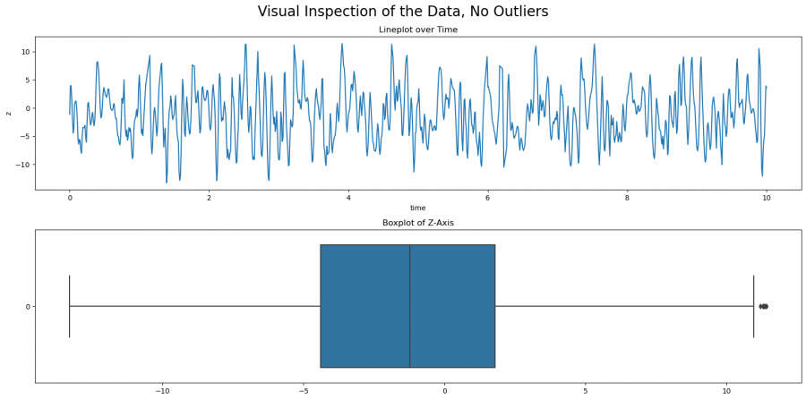
1. Completely remove outliers from the data set. The corresponding entries in the data set are not considered further in the analysis. However, it is not recommended to remove all outliers from data sets with many attributes, since potentially quite a lot of entries are removed across the different attributes. If you go back to the detection of outliers using IQR, you can easily identify the outliers and excluded them from the dataset (this works for all outlier detection methods, this one has been chosen as an example.
# Remove outliers based on IQR method
q1 = data['z'].quantile(0.25)
q3 = data['z'].quantile(0.75)
iqr = q3 - q1
upper_bound = q3 + 1.5 * iqr
lower_bound = q1 - 1.5 * iqr
data_no_outliers = data[(data['z'] > lower_bound) & (data['z'] < upper_bound)]

##check data
fig, axs = plt.subplots(2, figsize=(16, 8))
fig.suptitle('Visual Inspection of the Data, No Outliers', size=20)
sns.lineplot(data=data_no_outliers, x='time', y='z', ax=axs[0])
axs[0].set(title='Lineplot over Time')
sns.boxplot(data_no_outliers['z'], orient='h', ax=axs[1])
axs[1].set(title='Boxplot of Z-Axis')
plt.tight_layout()
plt.show()
Figure 6: Boxplot and line plot after the outliers have been removed
2. Alternatively, outliers can be replaced by NaN values and thus converted into missing values. However, it is recommended to perform the detection of outliers only on single attributes. The missing values can then be filled by value imputation methods.
# Calculate the IQR
Q1 = data['z'].quantile(0.25)
Q3 = data['z'].quantile(0.75)
IQR = Q3 - Q1

# Define the boundaries
lower_boundary = Q1 - 1.5 * IQR
upper_boundary = Q3 + 1.5 * IQR

# Replace outliers with NaN
data_nan = data.copy()
data_nan.loc[(data_nan['z'] < lower_boundary) | (data_nan['z'] > upper_boundary), 'z'] = np.nan
3. A third approach would be to keep the outliers and their respective values in the dataset but add a binary column that indicates whether a point is considered an outlier or not. When fitting models on the data, the model might learn to subtract a certain value for outliers. However, this approach is not the best-practice and should only be used if none of the above methods works well.
Key Publications
- P.A. MacMahon: The Expression of Syzygies among Perpetuants by Means of Partitions (1888) ([DOI](https://doi.org/10.2307/2369505 ) )
- Breunig et al.: LOF: identifying density-based local outliers (2000) ([DOI](https://doi.org/10.1145/335191.335388 ) )
- Prakhar Mishra: 5 Outlier Detection Techniques that every "Data Enthusiast" Must Know (2021) ([Link](https://towardsdatascience.com/5-outlier-detection-methods-that-every-data-enthusiast-must-know-f917bf439210))
The author of this entry is XX. Edited by Milan Maushart


