A matter of probability
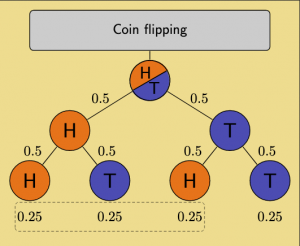
Probability indicates the likelihood whether something will occur or not. Typically, probabilities are represented by a number between zero and one, where one indicates the hundred percent probability that an event may occur, while zero indicates an impossibility of this event to occur.
The concept of probability goes way back to Arabian mathematicians and was initially strongly associated with cryptography. With rising recognition of preconditions that need to be met in order to discuss probability, concepts such as evidence, validity, and transferability were associated with probabilistic thinking. Probability plays also a role when it came to games, most importantly rolling dice. With the rise of the Enlightenment many mathematical underpinnings of probability were explored, most notably by the mathematician Jacob Bernoulli.
Gauss presented a real breakthrough, due to the discovery of the normal distribution. It allowed the feasible approach to link sample size of observations with an understanding of the likelihood how plausible these observations were. Again building on Sir Francis Bacon, the theory of probability reached its final breakthrough once it was applied in statistical hypothesis testing. It is important to notice that this would throw modern statistics into an understanding through the lens of so-called frequentist statistics. This line of thinking dominates up until today, and is widely built on repeated samples to understand the distribution of probabilities across a phenomenon.
Centuries ago, Thomas Bayes proposed a dramatically different approach. Here, an imperfect or a small sample would serve as basis for statistical interference. Very crudely defined, the two approaches start at exact opposite ends. While frequency statistics demand preconditions such as sample size and a normal distribution for specific statistical tests, Bayesian statistics build on the existing sample size; all calculations base on what is already there. Experts may excuse my dramatic simplification, but one could say that frequentist statistics are top-down thinking, while Bayesian statistics work bottom-up. The history of modern science is widely built on frequentist statistics, which includes such approaches as methodological design, sampling density and replicates, and diverse statistical tests. It is nothing short of a miracle that Bayes proposed the theoretical foundation for the theory named after him more than 250 years ago. Only with the rise of modern computers was this theory explored deeply, and builds the foundation of branches in data science and machine learning. The two approaches are also often coined as objectivists for frequentist probability fellows, and subjectivists for folllowers of Bayes theorem.
Another perspective on the two approaches can be built around the question whether we design studies - or whether we base our analysis on the data we just have. This debate is the basis for the deeply entrenched conflicts you have in statistics up until today, and was already the basis for the conflicts between Pearson and Fisher. From an epistemological perspective, this can be associated with the question of inductive or deductive reasoning, although not many statisticians might not be too keen to explore this relation deeply, since they are often stuck in either deductive or inductive thinking, but not both.
While probability today can be seen as one of the core foundations of statistical testing, probability as such is increasingly criticised. It would exceed this chapter to discuss this in depth, but let me just highlight that without understanding probability, much of the scientific literature building on quantitative methods is hard to understand. What is important to notice, is that probability has trouble considering Occam's razor. This is related to the fact that probability can deal well with the chance of an event to a occur, but it widely ignores the complexity that can influence such a likeliness. Modern statistics explore this thought further but let us just realise here: without learning probability we would have trouble reading the contemporary scientific literature.
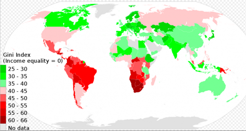
The probability can be best explained with the normal distribution. The normal distribution basically tells us through probability how a certain value will add to an array of values. Take the example of the height of people, or more specifically people who define themselves as males. Within a given population or country, these have an average height. This means in other words, that you have the highest chance to have this height when you are part of this population. You have a slightly lower chance to have a slightly smaller or larger height compared to the average height. And you have a very small chance to be much smaller or much taller compared to the average. In other words, your probability is small to be very tall or very small. Hence the distribution of height follows a normal distribution, and this normal distribution can be broken down into probabilities. In addition, such a distribution can have a variance, and these variances can be compared to other variances by using a so called f test. Take the example of height of people who define themselves as males. Now take the people who define themselves as females from the same population and compare just these two groups. You may realise that in most larger populations these two are comparable. This is quite relevant when you want to compare the income distribution between different countries. Many countries have different average incomes, but the distribution across the average as well as the very poor and the filthy rich can still be compared. In order to do this, the f-test is quite helpful.
#Let us perform a F test in R
#therefore we load the dataset 'women'

datasets::women
women_data<-women

#we want to compare the variances of height and weight for American women aged 30-39
#first we have to test for the normality of our samples

#q-q plots
qqnorm(women_data$height)
qqline(women_data$height)
qqnorm(women_data$weight)
qqline(women_data$weight)
#both are normally distributed


#F-Test (Test for Equality of Variance)
# H0 : Ratio of variance is equal to 1
# H1 : Ratio of variance is NOT equal to 1

var.test(women_data$height,women_data$weight)
#since p-value is low we reject H0
External Links
Websites
Seeing Theory: A great visual introduction to probability that you should definitely check out!
Articles
History of Probability: An Overview
Frequentist vs. Bayesian Approaches in Statistics: A comparison
Bayesian Statistics: An example from the wizarding world
Probability and the Normal Distribution: A detailed presentation
F test: An example in R
Compare your income: A tool by the OECD
Videos
Probability: An Introduction
Bayes Theorem: An explanation
F test: An example calculation
The author of this entry is Henrik von Wehrden.


