T-Test

In short: T-tests can be used to investigate whether there is a significant difference between two groups regarding a mean value (two-sample t-test) or the mean in one group compared to a fixed value (one-sample t-test). In the following article, the concept and purpose of the t-test, assumptions, the implementation in R as well as multiple variants for different conditions will be covered.

General Information

Let us start by looking at the basic idea behind a two-tailed two-sample t-test. Conceptually speaking we have two hypothesis:

H₀: Means between the two samples do not differ significantly. H₁: Means between the two samples do differ significantly.

In mathematical terms (μ₁ and μ₂ denote the mean values of the two samples):

H₀: μ₁ = μ₂
H₁: μ₁ ≠ μ₂.

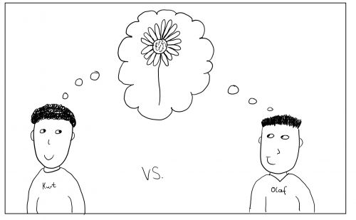
Here an example to illustrate this. The farmers Kurt and Olaf grow sunflowers and wonder who has the bigger ones. So they each measure a total of 100 flowers and put the values into a data frame.

# Create a dataset
set.seed(320)

kurt <- rnorm(100, 60.5, 22)
olaf <- rnorm(100, 63, 23)

Our task is now to find out whether means values differ significantly between two groups.

# perform t-test
t.test(kurt, olaf)


# Output:
## 
##  Welch Two Sample t-test
## 
## data:  kurt and olaf
## t = -1.5308, df = 192.27, p-value = 0.1275
## alternative hypothesis: true difference in means is not equal to 0
## 95 percent confidence interval:
##  -11.97670   1.50973
## sample estimates:
## mean of x mean of y 
##  57.77072  63.00421

Cool. We performed a t-test and got a result. But how can we interpret the output? The criterion to consult is the p-value. This value represents the probability of the data given that H0 is actually true. Hence, a low p-value indicates that the data is very unlikely if H0 applies. Therefore, one might reject this hypothesis (in favor of the alternative hypothesis H1) if the p-value turns out to be below a certain threshold (α , usually set prior testing), which is often set to 0.05 and usually not larger than 0.1. In this case, the p-value is greater than 0.1. Therefore, the probability of H0 is considered to be “too large” to reject this hypothesis. Hence, we conclude that means do not differ significantly, even though we can say that descriptively the sample mean of Olaf’s flowers is higher.

There are multiple options to fine-tune the t-test if one already has a concrete hypothesis in mind concerning the direction and/or magnitude of the difference. In the first case, one might apply a one-tailed t-test. The hypotheses pairs would change accordingly to either of these:

| H0: μ1 ≤ μ2

| H1: μ1 > μ2

Note that the hypotheses need to be mutually exclusive and H0 always contains some form of equality sign. In R, one-tailed testing is possible by setting alternative = "greater" or alternative = "less". Maybe Olaf is the more experienced farmer so we have already have à priori the hypothesis that his flowers are on average larger. This would refer to our alternative hypothesis. The code would change only slightly: