Difference between revisions of "Clustering Methods"
| Line 13: | Line 13: | ||
| style="width: 33%"| [[:Category:Past|Past]] || style="width: 33%"| '''[[:Category:Present|Present]]''' || [[:Category:Future|Future]] | | style="width: 33%"| [[:Category:Past|Past]] || style="width: 33%"| '''[[:Category:Present|Present]]''' || [[:Category:Future|Future]] | ||
|} | |} | ||
| + | <br/> | ||
<br/> | <br/> | ||
<br/> | <br/> | ||
Revision as of 08:55, 7 December 2020
| Method categorization | ||
|---|---|---|
| Quantitative | Qualitative | |
| Inductive | Deductive | |
| Individual | System | Global |
| Past | Present | Future |
In short: Clustering is a method of data analysis through the grouping of unlabeled data based on certain metric.
Contents
Background
Cluster analysis shares history in various fields such as anthropology, psychology, biology, medicine, business, computer science, and social science.
It originated in anthropology when Driver and Kroeber published Quantitative Expression of Cultural Relationships in 1932 where they sought to clusters of culture based on different culture elements. Then, the method was introduced to psychology in the late 1930s.
What the method does
Clustering is a method of grouping unlabeled data based on certain metric, often referred to as similarity measure or distance measure, such that the data points within each cluster are similar to each other, and any points that lie in separate cluster are dissimilar. Clustering is a statistical method that falls under a class of Machine Learning algorithms named "unsupervised learning", although clustering is also performed in many other fields such as data compression, pattern recognition, etc. Finally, the term "clustering" does not refer to a specific algorithm, but rather a family of algorithms; the similarity measure employed to perform clustering depends on specific clustering model.
While there are many clustering methods, two common approaches are discussed in this article.
Data Simulation
This article deals with simulated data. This section contains the function used to simulate the data. For the purpose of this article, the data has three clusters. You need to load the function on your R environment in order to simulate the data and perform clustering.
create_cluster_data <- function(n=150, sd=1.5, k=3, random_state=5){
    # currently, the function only produces 2-d data

    # n = no. of observation
    # sd = within-cluster sd
    # k = number of clusters
    # random_state = seed

    set.seed(random_state)
    dims = 2 # dimensions
    xs = matrix(rnorm(n*dims, 10, sd=sd), n, dims)
    clusters = sample(1:k, n, replace=TRUE)
    centroids = matrix(rnorm(k*dims, mean=1, sd=10), k, dims)
    clustered_x = cbind(xs + 0.5*centroids[clusters], clusters)

    plot(clustered_x, col=clustered_x[,3], pch=19)

    df = as.data.frame(x=clustered_x)
    colnames(df) <- c("x1", "x2", "cluster")
    return(df)
}
k-Means Clustering
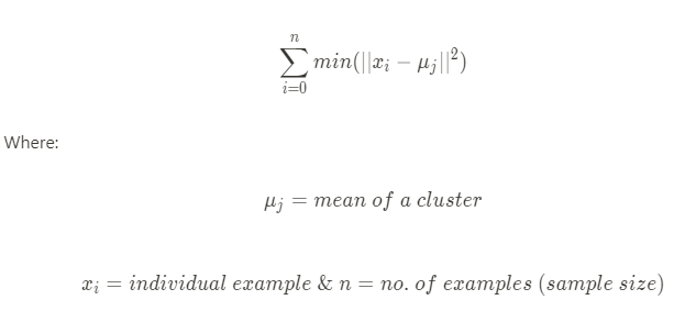
The k-means clustering method assigns n examples to one of k clusters, where n is the sample size and k, which needs to be chosen before the algorithm is implemented, is the number of clusters. This clustering method falls under a clustering model called centroid model where centroid of a cluster is defined as the mean of all the points in the cluster. K-means Clustering algorithm aims to choose centroids that minimize the within-cluster sum-of-squares criterion based on the following formula:
The in-cluster sum-of-squares is also called inertia in some literature.
The algorithm involves following steps:
- The number of cluster k is chosen by the data analyst
- The algorithm randomly picks k centroids and assigns each point to the closest centroid to get k initial clusters
- The algorithm recalculates the centroid by taking average of all points in each cluster and updates the centroids and re-assigns the points to the closest centroid.
- The algorithm repeats Step 3 until all points stop changing clusters.
To get an intuitive sense of how this k-means clustering algorithm works, visit: Visualizing K-Means Clustering
Implementing k-Means Clustering in R
To implement k-Means Clustering, the data table needs to only contain numeric data type. With a data frame or matrix with numeric value where the rows signify individual data example and the columns signify the features (number of features = the number of dimensions of the data set), k-Means clustering can be performed with the code below:
# Generate data and perform the clustering
df <- create_cluster_data(150, 1.25, 3)
data_cluster = kmeans(df, centers=3) # perform the clustering

# plot for sd = 1.25
plot(df$x1, df$x2,
     pch=df$cluster,
     col=data_cluster$cluster, cex=1.3,
     xlab="x1", ylab="x2",
     main="k-Means Clustering Example with Clearly Clustered Data",
     sub="(In-cluster variance when generating data = 1.25)")
points(data_cluster$centers[1,1], data_cluster$centers[1,2],
       pch=15, cex=2, col="black")
points(data_cluster$centers[2,1], data_cluster$centers[2,2],
       pch=15, cex=2, col="red")
points(data_cluster$centers[3,1], data_cluster$centers[3,2],
       pch=15, cex=2, col="green")
legend("topleft", legend=c("True Cluster 1", "True Cluster 2", "True Cluster 3", "Cluster Center"),
       col=c("black","black","black", "black"), pch = c(1, 2, 3, 15), cex=0.8)
text(-3.15, 10,
     "Colors signify the clusters identified\nby k-means clustering algorithm",
     adj = c(0,0), cex=0.8)
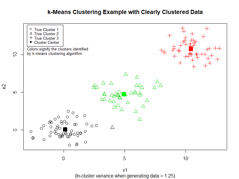
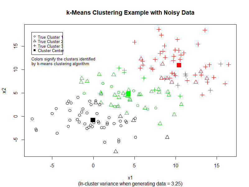
Here is the result of the preceding code:
We can see that k-Means performs quite good at separating the data into three clusters. However, if we increase the variance in the dataset, k-Means does not perform as well. (See image below)
Strengths and Weaknesses of k-Means Clustering
Strengths
- It is intuitive to understand.
- It is relatively easy to implement.
- It adapts to new data points and guarantees convergence.
Weaknesses
- The number of clusters *k* has to be chosen manually.
- The vanilla k-Means algorithm cannot accommodate cases with a high number of clusters (high *k*).
- The k-Means clustering algorithm clusters *all* the data points. As a result, the centroids are affected by outliers.
- As the dimension of the dataset increases, the performance of the algorithm starts to deteriorate.
Hierarchical Clustering
As the name suggests, hierarchical clustering is a clustering method that builds a *hierarchy* of clusters.
Unlike k-Means clustering algorithm discussed above, this clustering method does not require us to specify the number of clusters beforehand. As a result, this method is sometimes used to identify the number of clusters that a dataset has before applying other clustering algorithms that require us to specify the number of clusters at the beginning.
There are two strategies when performing hierarchical clustering:
Hierarchical Agglomerative Clustering
This is a "bottom-up" approach of building hierarchy which starts by treating each data point as a single cluster, and successively merging pairs of clusters, or agglomerating, until all clusters have been merged into a single cluster that contains all data points.
- Each observation belongs to its own cluster, then pairs of clusters are merged as one moves up the hierarchy.
Implementation of Agglomerative Clustering
The first example of agglomerative clustering is performed using the hclust function built in to R.
library(dendextend)

# generate data
df <- create_cluster_data(50, 1, 3, random_state=7)
# create the distance matrix
dist_df = dist(df[, 2], method="euclidean")
# perform agglomerative hierarchical clustering
hc_df = hclust(dist_df, method="complete")
# create a simple plot of the dendrogram
plot(hc_df)

# Plot a more sophisticated version of the dendrogram
dend_df <- as.dendrogram(hc_df)
dend_df <- rotate(dend_df, 1:50)
dend_df <- color_branches(dend_df, k=3)
labels_colors(dend_df) <-
    c("black", "darkgreen", "red")[sort_levels_values(
        as.numeric(df[,3])[order.dendrogram(dend_df)])]
labels(dend_df) <- paste(as.character(
    paste0("cluster_",df[,3]," "))[order.dendrogram(dend_df)],
    "(",labels(dend_df),")",
    sep = "")
dend_df <- hang.dendrogram(dend_df, hang_height=0.2)
dend_df <- set(dend_df, "labels_cex", 0.8)

plot(dend_df,
     main = "Clustered Data Set
     (based on Agglomerative Clustering using hclust() function)",
     horiz =  FALSE,  nodePar = list(cex = 0.5), cex=1)

legend("topleft",
       legend = c("Cluster 1", "Cluster 2", "Cluster 3"),
       fill = c("darkgreen", "black", "red"))
Here is the plot of the dendrogram from the code above:
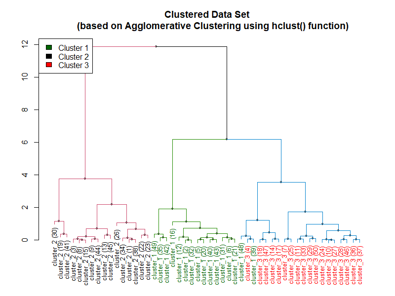
The following example relies on the agnes function from cluster package in R in order to preform agglomerative hierarchical clustering.
df <- create_cluster_data(50, 1, 3, random_state=7)
dend_df <- agnes(df, metric="euclidean")

# Plot the dendrogram
dend_df <- as.dendrogram(dend_df)
dend_df <- rotate(dend_df, 1:50)
dend_df <- color_branches(dend_df, k=3)
labels_colors(dend_df) <-
    c("black", "darkgreen", "red")[sort_levels_values(
        as.numeric(df[,3])[order.dendrogram(dend_df)])]
labels(dend_df) <- paste(as.character(
    paste0("cluster_",df[,3]," "))[order.dendrogram(dend_df)],
    "(",labels(dend_df),")",
    sep = "")
dend_df <- hang.dendrogram(dend_df,hang_height=0.2)
dend_df <- set(dend_df, "labels_cex", 0.8)

plot(dend_df,
     main = "Clustered Data Set
     (based on Agglomerative Clustering using agnes() function)",
     horiz =  FALSE,  nodePar = list(cex = 0.5), cex=1)
legend("topleft",
       legend = c("Cluster 1", "Cluster 2", "Cluster 3"),
       fill = c("darkgreen", "black", "red"))
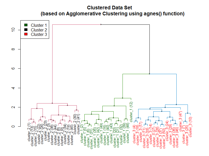
Following is the dendrogram created using the preceding code:
Hierarchical Divisive Clustering
This is a "top-down" approach of building hierarchy in which all data points start out as belonging to a single cluster. Then, the data points are split, or divided, into separate clusters recursively until each of them falls into its own separate individual clusters.
- All observations start as one cluster, and splits are performed recursively as one moves down the hierarchy.
Implementation of Divisive Clustering
# Generate a dataset
df <- create_cluster_data(50, 1, 3, random_state=7)

# Perform divisive clustering
dend_df <- diana(df, metric="euclidean")

# Plot the dendrogram
dend_df <- as.dendrogram(dend_df)
dend_df <- rotate(dend_df, 1:50)
dend_df <- color_branches(dend_df, k=3)

labels_colors(dend_df) <-
    c("black", "darkgreen", "red")[sort_levels_values(
        as.numeric(df[,3])[order.dendrogram(dend_df)])]

labels(dend_df) <- paste(as.character(
    paste0("cluster_",df[,3]," "))[order.dendrogram(dend_df)],
    "(",labels(dend_df),")",
    sep = "")

dend_df <- hang.dendrogram(dend_df, hang_height=1) # 0.1
dend_df <- set(dend_df, "labels_cex", 0.8)

plot(dend_df,
     main = "Clustered Data Set
     (based on Divisive Clustering using diana() function)",
     horiz =  FALSE,  nodePar = list(cex = 0.5), cex=1)
legend("topleft",
       legend = c("Cluster 1", "Cluster 2", "Cluster 3"),
       fill = c("darkgreen", "black", "red"))
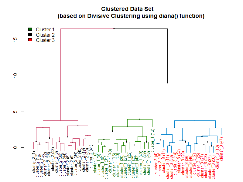
Following is the result of the code above:
Strengths and Weaknesses of Hierarchical Clustering
Strengths
- The method does not require users to pre-specify the number of clusters manually.
- This method does not work account for missing values.
Weaknesses
- Even though the number of clusters does not have to be pre-specified, users still need to specify the *distance metric* and the *linkage criteria*.
- This method becomes very slow when the size of the data set is large.
See Also
Although this article only focused on two clustering algorithms. There are many other clustering methods that employ different strategies. Readers are suggested to investigate expectation maximization algorithm, and density based clustering algorithms, and latent class analysis specifically.
Key Publications
k-Means Clustering
- MacQueen, James. "Some methods for classification and analysis of multivariate observations." Proceedings of the fifth Berkeley symposium on mathematical statistics and probability. Vol. 1. No. 14. 1967.
Hierarchical Clustering
- Johnson, S.C. Hierarchical clustering schemes. Psychometrika 32, 241–254 (1967). [1](https://doi.org/10.1007/BF02289588)
- Murtagh, F., & Legendre, P. (2014). Ward’s hierarchical agglomerative clustering method: which algorithms implement Ward’s criterion?. Journal of classification, 31(3), 274-295.
Other Clustering Methods
- A. K. Jain, M. N. Murty, and P. J. Flynn. 1999. Data clustering: a review. ACM Comput. Surv. 31, 3 (September 1999), 264–323. DOI:[2](https://doi.org/10.1145/331499.331504)
- Lanza, S. T., & Rhoades, B. L. (2013). Latent class analysis: an alternative perspective on subgroup analysis in prevention and treatment. Prevention science : the official journal of the Society for Prevention Research, 14(2), 157–168. [3](https://doi.org/10.1007/s11121-011-0201-1)
- Erich Schubert, Jörg Sander, Martin Ester, Hans Peter Kriegel, and Xiaowei Xu. 2017. DBSCAN Revisited, Revisited: Why and How You Should (Still) Use DBSCAN. ACM Trans. Database Syst. 42, 3, Article 19 (July 2017), 21 pages. DOI:[4](https://doi.org/10.1145/3068335)
The author of this entry is Prabesh Dhakal.
