Difference between revisions of "Support Vector Machine in Python"
(Created page with "THIS ARTICLE IS STILL IN EDITING MODE ==Introduction== Support Vector Machine (SVM) is a supervised machine learning algorithm which uses supervised learning models to solve...") |
|||
| Line 294: | Line 294: | ||
The author of this entry is Bhavana Raju. Edited by Evgeniya Zakharova. | The author of this entry is Bhavana Raju. Edited by Evgeniya Zakharova. | ||
| − | |||
| − | |||
| − | |||
| − | |||
Latest revision as of 13:40, 3 September 2024
THIS ARTICLE IS STILL IN EDITING MODE
Contents
Introduction
Support Vector Machine (SVM) is a supervised machine learning algorithm which uses supervised learning models to solve complex classification, regression, and outlier detection problems by performing optimal data transformations that determine boundaries between data points based on predefined classes, labels, or outputs. However, it is mostly used in classification problems. Introduced by Vapnik and Cortes in the 1990s, SVMs have gained immense popularity due to their ability to handle high-dimensional data and their robust performance in a variety of applications.
Note: Do not get confused between SVM and logistic regression. Both algorithms try to find the best hyperplane, but the main difference is, that logistic regression is a probabilistic approach, whereas SVMs are based on statistical approaches.
Logistic Regression VS Support Vector Machine
Depending on the number of features we can either choose Logistics Regression or SVM. SVM works best when the dataset is small and complex. It is often advised, first to use logistic regression and see how it performs, if it fails to give a good accuracy, then SVM can be applied. Logistic Regression and SVM without any kernels have similar performance, but depending on the features, one may be more efficient than the other.
Types of Support Vector Machine Algorithms
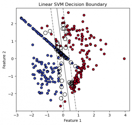
Linear SVM
If the data is perfectly linearly separable, Linear SVM can be utilized. Perfectly linearly separable means that the data points can be classified into 2 classes by using a single straight line (if 2D).
Importing libraries and creating dataset
# Importing libraries
import numpy as np
import matplotlib.pyplot as plt
from sklearn.datasets import make_classification
from sklearn.model_selection import train_test_split
from sklearn.preprocessing import StandardScaler
from sklearn.svm import SVC
from sklearn.metrics import accuracy_score, confusion_matrix, classification_report

# Creating a synthetic dataset
X, y = make_classification(n_samples=300, n_features=2, n_informative=2, n_redundant=0, random_state=42)

# Spliting the data into training and testing sets
X_train, X_test, y_train, y_test = train_test_split(X, y, test_size=0.2, random_state=42)

# Standardizing features
scaler = StandardScaler()
X_train = scaler.fit_transform(X_train)
X_test = scaler.transform(X_test)
# Linear SVM
linear_svm_model = SVC(kernel='linear', C=1.0)

# Training the Linear SVM model
linear_svm_model.fit(X_train, y_train)

# Making predictions on the test set
y_pred_linear = linear_svm_model.predict(X_test)

# Calculating the accuracy of the linear model
accuracy_linear = accuracy_score(y_test, y_pred_linear)
print(f"Linear SVM Accuracy: {accuracy_linear:.2f}")

# Displaying confusion matrix and classification report for the linear model
conf_matrix_linear = confusion_matrix(y_test, y_pred_linear)
class_report_linear = classification_report(y_test, y_pred_linear)

print("\nConfusion Matrix (Linear SVM):")
print(conf_matrix_linear)
print("\nClassification Report (Linear SVM):")
print(class_report_linear)
Linear SVM Accuracy: 0.92
Confusion Matrix (Linear SVM):
[[27 3]
[2 28]]
Classification Report (Linear SVM):
| precision | recall | f1-score | support | |
|---|---|---|---|---|
| 0 | 0.93 | 0.90 | 0.92 | 30 |
| 1 | 0.90 | 0.93 | 0.92 | 30 |
| accuracy | 0.92 | 60 | ||
| macro avg | 0.92 | 0.92 | 0.92 | 60 |
| weighted avg | 0.92 | 0.92 | 0.92 | 60 |
# Visualizing decision boundaries
plt.figure(figsize=(12, 5))

# Plotting Linear SVM Decision Boundary
plt.subplot(1, 2, 1)
plt.scatter(X[:, 0], X[:, 1], c=y, cmap=plt.cm.coolwarm, edgecolors='k')
plt.title('Linear SVM Decision Boundary')
ax = plt.gca()
xlim = ax.get_xlim()
ylim = ax.get_ylim()

# Creating grid to evaluate model
xx, yy = np.meshgrid(np.linspace(xlim[0], xlim[1], 50),
                     np.linspace(ylim[0], ylim[1], 50))
Z = linear_svm_model.decision_function(np.c_[xx.ravel(), yy.ravel()])
Z = Z.reshape(xx.shape)

# Plotting decision boundary and margins
plt.contour(xx, yy, Z, colors='k', levels=[-1, 0, 1], alpha=0.5,
            linestyles=['--', '-', '--'])
plt.scatter(linear_svm_model.support_vectors_[:, 0], linear_svm_model.support_vectors_[:, 1],
            s=100, facecolors='none', edgecolors='k')
plt.xlabel('Feature 1')
plt.ylabel('Feature 2')
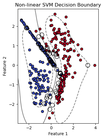
Non-Linear SVM
If the data is not linearly separable, we can use Non-Linear SVM, which means when the data points cannot be separated into 2 classes by using a straight line (if 2D), then we use some advanced techniques (like kernel tricks) to classify them. In most real-world applications we do not find linearly separable data points, hence we use kernel tricks to solve them. (We will use the same libraries and dataset for this example, as for Linnear SVM).
# Non-linear SVM with RBF kernel
non_linear_svm_model = SVC(kernel='rbf', C=1.0, gamma='scale')

# Training the Non-linear SVM model
non_linear_svm_model.fit(X_train, y_train)

# Making predictions on the test set
y_pred_non_linear = non_linear_svm_model.predict(X_test)

# Calculating the accuracy of the non-linear model
accuracy_non_linear = accuracy_score(y_test, y_pred_non_linear)
print(f"\nNon-linear SVM Accuracy: {accuracy_non_linear:.2f}")

# Displaying confusion matrix and classification report for the non-linear model
conf_matrix_non_linear = confusion_matrix(y_test, y_pred_non_linear)
class_report_non_linear = classification_report(y_test, y_pred_non_linear)

print("\nConfusion Matrix (Non-linear SVM):")
print(conf_matrix_non_linear)
print("\nClassification Report (Non-linear SVM):")
print(class_report_non_linear)
Non-linear SVM Accuracy: 0.97
Confusion Matrix (Non-linear SVM):
[[29 1]
[1 29]]
Classification Report (Non-linear SVM):
| precision | recall | f1-score | support | |
|---|---|---|---|---|
| 0 | 0.97 | 0.97 | 0.97 | 30 |
| 1 | 0.97 | 0.97 | 0.97 | 30 |
| accuracy | 0.97 | 60 | ||
| macro avg | 0.97 | 0.97 | 0.97 | 60 |
| weighted avg | 0.97 | 0.97 | 0.97 | 60 |
# Plotting Non-linear SVM Decision Boundary
plt.subplot(1, 2, 2)
plt.scatter(X[:, 0], X[:, 1], c=y, cmap=plt.cm.coolwarm, edgecolors='k')
plt.title('Non-linear SVM Decision Boundary')
ax = plt.gca()
xlim = ax.get_xlim()
ylim = ax.get_ylim()

# Creating grid to evaluate model
xx, yy = np.meshgrid(np.linspace(xlim[0], xlim[1], 50),
                     np.linspace(ylim[0], ylim[1], 50))
Z = non_linear_svm_model.decision_function(np.c_[xx.ravel(), yy.ravel()])
Z = Z.reshape(xx.shape)

# Plotting decision boundary and margins
plt.contour(xx, yy, Z, colors='k', levels=[-1, 0, 1], alpha=0.5,
            linestyles=['--', '-', '--'])
plt.scatter(non_linear_svm_model.support_vectors_[:, 0], non_linear_svm_model.support_vectors_[:, 1],
            s=100, facecolors='none', edgecolors='k')
plt.xlabel('Feature 1')
plt.ylabel('Feature 2')

plt.tight_layout()
plt.show()
Hyperplane
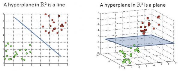
Hyperplanes are decision boundaries that help classify the data points. Data points falling on either side of the hyperplane can be attributed to different classes. Also, the dimension of the hyperplane depends upon the number of features. If the number of input features is 2, then the hyperplane is just a line. If the number of input features is 3, then the hyperplane becomes a two-dimensional plane. It becomes difficult to imagine the featere space when their number exceeds 3. Examples of hyperplane in 2D and 3D feature space are presented in Figure 1.
Support Vectors and Margin
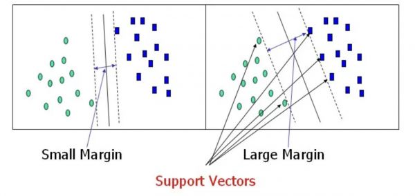
Support Vectors are the points, which are the closest to the hyperplane. A separating line will be defined with the help of these data points.
Margin is the distance between the hyperplane and the observations, which are the closest to the hyperplane (support vectors). In SVM large margin is considered as a good margin (Figure 2).
Large Margin Intuition
In logistic regression, we take the output of the linear function and squash the value within the range of [0,1] using the sigmoid function. If the squashed value is greater than a threshold value (0.5) we assign it a label 1, otherwise, we assign it a label 0. In SVM, we take the output of the linear function and if that output is greater than 1, we identify it with one class and if the output is -1, we identify it with another class. Since the threshold values are changed to 1 and -1 in SVM, we obtain this reinforcement range of values [-1,1], which acts as margin.
Loss Function
In the SVM algorithm, we are trying to maximise the margin between the data points and the hyperplane. The loss function that helps maximise the margin is hinge loss: L(y, f(x)) = max(0, 1-y*f(x)), where y is a class of the data point (-1,1) and f(x) is an output of the model.
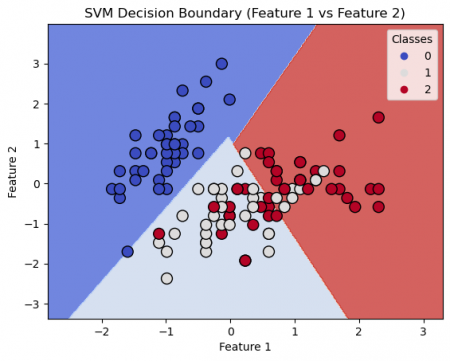
SVM Example - IRIS dataset
# Importing necessary libraries
import numpy as np
import matplotlib.pyplot as plt
from sklearn import datasets
from sklearn.model_selection import train_test_split
from sklearn.preprocessing import StandardScaler
from sklearn.svm import SVC
from sklearn.metrics import accuracy_score

# Loading the Iris dataset
iris = datasets.load_iris()
X = iris.data[:, :2]  # Using only the first two features for visualization
y = iris.target

# Spliting the dataset into training and testing sets
X_train, X_test, y_train, y_test = train_test_split(X, y, test_size=0.2, random_state=42)

# Standardizing features
scaler = StandardScaler()
X_train = scaler.fit_transform(X_train)
X_test = scaler.transform(X_test)

# Creating an SVM model
svm_model = SVC(kernel='linear', C=1.0)

# Training the SVM model
svm_model.fit(X_train, y_train)

# Making predictions on the test set
y_pred = svm_model.predict(X_test)

# Evaluating the model
accuracy = accuracy_score(y_test, y_pred)
print(f"Accuracy: {accuracy:.2f}")
Accuracy: 0.90
# Plotting decision boundary
def plot_decision_boundary(X, y, model, title):
    h = .02  # step size in the mesh
    x_min, x_max = X[:, 0].min() - 1, X[:, 0].max() + 1
    y_min, y_max = X[:, 1].min() - 1, X[:, 1].max() + 1
    xx, yy = np.meshgrid(np.arange(x_min, x_max, h), np.arange(y_min, y_max, h))

    Z = model.predict(np.c_[xx.ravel(), yy.ravel()])
    Z = Z.reshape(xx.shape)

    plt.contourf(xx, yy, Z, cmap=plt.cm.coolwarm, alpha=0.8)
    scatter = plt.scatter(X[:, 0], X[:, 1], c=y, cmap=plt.cm.coolwarm, edgecolors='k', s=100)
    plt.legend(*scatter.legend_elements(), title="Classes")
    plt.title(title)
    plt.xlabel('Feature 1')
    plt.ylabel('Feature 2')
    plt.show()

# Plotting decision boundary
plot_decision_boundary(X_train, y_train, svm_model, 'SVM Decision Boundary (Feature 1 vs Feature 2)')
Refereces
1. https://scikit-learn.org/stable/modules/svm.html
2. https://www.analyticsvidhya.com/blog/2017/09/understaing-support-vector-machine-example-code/
3. https://www.spiceworks.com/tech/big-data/articles/what-is-support-vector-machine/
The author of this entry is Bhavana Raju. Edited by Evgeniya Zakharova.
