Difference between revisions of "Data Transformation"
Oskarlemke (talk | contribs) |
|||
| (9 intermediate revisions by one other user not shown) | |||
| Line 6: | Line 6: | ||
This transformation builds on the logarithm, which is the exponent to which a certain number (the base) has to be raised to result in a given number. | This transformation builds on the logarithm, which is the exponent to which a certain number (the base) has to be raised to result in a given number. | ||
| − | '''Example:''' 10 | + | '''Example:''' 10<sup>2</sup>=100 so the logarithm would be 2=log<sub>10</sub>(100) |
Logarithms with base 10 are called common logarithms, with a base of 2 they are called binary logarithms and natural logarithms are those with the base “e” (Euler’s number). | Logarithms with base 10 are called common logarithms, with a base of 2 they are called binary logarithms and natural logarithms are those with the base “e” (Euler’s number). | ||
| Line 15: | Line 15: | ||
The following example shows the use of a log transformation for a variable of the swiss dataset in Rstudio. The data for the variable Education is not close to following a normal distribution, but the log transformed data is closer to being normally distributed, as observable in the histograms. When linear models are made to look at the relationship between the variables Education and Examination, the residuals of the linear model with the original data do not follow a normal distribution, while the residuals of the model with the log transformed data do. | The following example shows the use of a log transformation for a variable of the swiss dataset in Rstudio. The data for the variable Education is not close to following a normal distribution, but the log transformed data is closer to being normally distributed, as observable in the histograms. When linear models are made to look at the relationship between the variables Education and Examination, the residuals of the linear model with the original data do not follow a normal distribution, while the residuals of the model with the log transformed data do. | ||
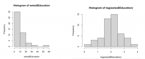
| − | [[File: | + | [[File:Histograms swiss$Education.png|480px|thumb|left|As you can see, the data does not follow a normal distribution, but the log transformed data is much closer to following a normal distribution.]] |
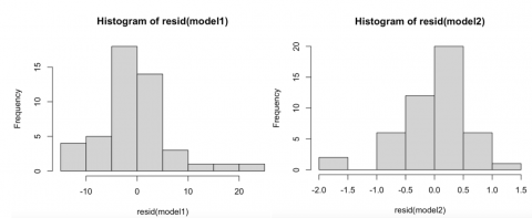
| − | [[File: | + | [[File:Histograms Models swiss$Education.png|480px|thumb|left|The residuals from Model 1 do not follow a normal distribution, while the residuals from Model 2 with the log transformed data are closer to being normally distributed.]] |
| − | + | ||
str(swiss) | str(swiss) | ||
par(mfrow=c(2,3)) | par(mfrow=c(2,3)) | ||
| Line 33: | Line 33: | ||
hist(resid(model1)) | hist(resid(model1)) | ||
hist(resid(model2)) | hist(resid(model2)) | ||
| − | |||
| − | |||
==External Sources== | ==External Sources== | ||
Latest revision as of 10:49, 7 July 2024
Contents
Data Transformation
Frequentist statistics typically build on statistical distributions, making it necessary not only to check data for their distribution, but also to transform the data to meet a certain distribution. The normal distribution stands out as the fundamental basis of many simple statistical models, making it necessary to transform data in order to meet the preconditions of respective models. In this entry we will look at several statistical distributions, and discuss the steps necessary if you encounter skewed distributions.
Log Transformation
A very common data transformation is the so-called log transformation, which is typically applied to count data, which more often than not has a tendency to have the majority of the data on the low end of the counts, and few high counts. Be careful though, count data in the form of response variables should not be log transformed, this can skew the results, especially when the data includes ‘zero’ observations. This transformation builds on the logarithm, which is the exponent to which a certain number (the base) has to be raised to result in a given number.
Example: 102=100 so the logarithm would be 2=log10(100) Logarithms with base 10 are called common logarithms, with a base of 2 they are called binary logarithms and natural logarithms are those with the base “e” (Euler’s number).
Using the log transformation
The common use of the log transformation is to transform continuous data that does originally not follow the normal distribution into a reformatting that at least more closely meets the normal distribution, thereby reducing the skewness of the data. The transformed data then ideally meets the criteria of the normal distribution. However, this will only work if the original data follows a log-normal distribution in order for a log transformation to work and thus enable the possibility to apply the respective statistical analysis. With a log transformation you reformat your data into its logarithmic values by taking the logarithm of each value. Then your data should follow a normal distribution, because a lot of data follows a log-normal distribution.
R Example
The following example shows the use of a log transformation for a variable of the swiss dataset in Rstudio. The data for the variable Education is not close to following a normal distribution, but the log transformed data is closer to being normally distributed, as observable in the histograms. When linear models are made to look at the relationship between the variables Education and Examination, the residuals of the linear model with the original data do not follow a normal distribution, while the residuals of the model with the log transformed data do.
str(swiss)
par(mfrow=c(2,3))
for(i in 1:6){
hist(swiss[,i])
}
round(cor(swiss),d=2)
par(mfrow=c(1,2))
hist(swiss$Education)
hist(log(swiss$Education))
model1<-lm(swiss$Education~swiss$Examination)
summary(model1)
model2<-lm(log(swiss$Education)~swiss$Examination)
summary(model2)
hist(resid(model1))
hist(resid(model2))
External Sources
Htoon, K.S. (2020). Log Transformation: Purpose and Interpretation. Accessed through https://medium.com/@kyawsawhtoon/log-transformation-purpose-and-interpretation-9444b4b049c9
O’Hara, R., Kotze, J. (2010). Do not log-transform count data. Methods in Ecology and Evolution, 1(2):118-122.
Yudha Wijaya, C. (2021). Beginner Explanation for Data Transformation. Accessed through https://towardsdatascience.com/beginner-explanation-for-data-transformation-9add3102f3bf
The author of this entry is Melissa Figiel.

