Difference between revisions of "Ancova"
m |
Oskarlemke (talk | contribs) |
||
| (4 intermediate revisions by 2 users not shown) | |||
| Line 5: | Line 5: | ||
'''Prerequisite knowledge''' | '''Prerequisite knowledge''' | ||
| − | An understanding of ANOVA | + | An understanding of the [[ANOVA]] |
* Main effects and interaction effects | * Main effects and interaction effects | ||
* Sum of squares | * Sum of squares | ||
| Line 18: | Line 18: | ||
== Definition == | == Definition == | ||
| − | Analysis of covariance (ANCOVA) is the statistical test that compares the means of more than two groups by taking under the control the "noise" caused by covariate variable that is not of experimental interest. This is done in order to see the true effect of the variable of interest on a dependent variable. Fundamental idea of ANCOVA is based on hypothesis testing, its goal is to evaluate multiple mutually exclusive theories about our data, where null hypothesis claims that the means of the groups are equal, and alternative hypothesis rejects that based on p-value. Additionally, it is important to highlight that ANCOVA also gives information on variables by means of Sum of Squares partitioning that shows the size of error or unexplained information in relation. Since ANCOVA historically comes from the combination of Linear regression and ANOVA, one should meet the assumptions inherent from them as well as specific to ANCOVA before proceeding to the ANCOVA test. | + | Analysis of covariance (ANCOVA) is the statistical test that compares the means of more than two groups by taking under the control the "noise" caused by covariate variable that is not of experimental interest. This is done in order to see the true effect of the variable of interest on a dependent variable. Fundamental idea of ANCOVA is based on hypothesis testing, its goal is to evaluate multiple mutually exclusive theories about our [[Glossary|data]], where null hypothesis claims that the means of the groups are equal, and alternative [[Glossary|hypothesis]] rejects that based on p-value. Additionally, it is important to highlight that ANCOVA also gives information on variables by means of Sum of Squares partitioning that shows the size of error or unexplained information in relation. Since ANCOVA historically comes from the combination of Linear regression and ANOVA, one should meet the assumptions inherent from them as well as specific to ANCOVA before proceeding to the ANCOVA test. |
| + | |||
== Assumptions == | == Assumptions == | ||
'''Regression assumptions''' | '''Regression assumptions''' | ||
| Line 27: | Line 28: | ||
'''Specific ANCOVA assumptions''' | '''Specific ANCOVA assumptions''' | ||
# A further specific (but optional) assumption is homogeneity of slopes. It is optional because it is only required to simplify the model for estimation of adjusted means. | # A further specific (but optional) assumption is homogeneity of slopes. It is optional because it is only required to simplify the model for estimation of adjusted means. | ||
| + | |||
==What is One-way ANCOVA?== | ==What is One-way ANCOVA?== | ||
| − | One-way ANCOVA compares the variance in the group means within a sample with only one independent variable or factor that has three or more than three categorical groups whilst considering the | + | One-way ANCOVA compares the variance in the group means within a sample with only one independent variable or factor that has three or more than three categorical groups whilst considering the covariate. Since ANCOVA is hypothesis-based test, we need to have a understanding and well developed question about our data that we want an answer to, before we can generate a hypothesis and run the test. |
| + | |||
===Data preparation=== | ===Data preparation=== | ||
| Line 38: | Line 41: | ||
#installing the package datarium where we can find different types of datasets | #installing the package datarium where we can find different types of datasets | ||
</syntaxhighlight> | </syntaxhighlight> | ||
| + | |||
===Exploring the data=== | ===Exploring the data=== | ||
| Line 68: | Line 72: | ||
Based on the boxplot we can see that the anxiety mean score is the highest for individuals who have been practicing basal(grp1) type of exercises and the lowest for individuals who have been practicing the high(grp3) type of exercises. These observations are made based on descriptive statistic by not taking into consideration the overall personal ability of each individual to control his/her anxiety level, let us prove it statistically with the help of ANCOVA. | Based on the boxplot we can see that the anxiety mean score is the highest for individuals who have been practicing basal(grp1) type of exercises and the lowest for individuals who have been practicing the high(grp3) type of exercises. These observations are made based on descriptive statistic by not taking into consideration the overall personal ability of each individual to control his/her anxiety level, let us prove it statistically with the help of ANCOVA. | ||
| − | |||
| + | ===Checking assumptions=== | ||
1. Linearity assumption can be assessed with the help of the regression fitted lines plot for each treatment group. Based on the plot bellow we can visually assess that the relationship between anxiety score before and after treatment is linear. | 1. Linearity assumption can be assessed with the help of the regression fitted lines plot for each treatment group. Based on the plot bellow we can visually assess that the relationship between anxiety score before and after treatment is linear. | ||
[[File:Score_by_the_treatment_type2.png|250px|thumb|left|alt text]] | [[File:Score_by_the_treatment_type2.png|250px|thumb|left|alt text]] | ||
| Line 179: | Line 183: | ||
---- | ---- | ||
[[Category:Statistics]] | [[Category:Statistics]] | ||
| + | [[Category:R examples]] | ||
Latest revision as of 10:22, 14 June 2024
In short: Analysis of covariance (ANCOVA) is a statistical test that compares the means of more than two groups by taking under the control the "noise" caused by covariate variable that is not of experimental interest. This is done in order to see the true effect of the variable of interest on a dependent variable.
Contents
Prerequites
Prerequisite knowledge An understanding of the ANOVA
- Main effects and interaction effects
- Sum of squares
- Mean squares
- ANOVA tables
- F-statistics and significance values
- Post-hoc analysis (Tukey, Bonferonni, etc.)
An understanding of Linear Regression
- Regression slopes
- p-values
- Coefficients
Definition
Analysis of covariance (ANCOVA) is the statistical test that compares the means of more than two groups by taking under the control the "noise" caused by covariate variable that is not of experimental interest. This is done in order to see the true effect of the variable of interest on a dependent variable. Fundamental idea of ANCOVA is based on hypothesis testing, its goal is to evaluate multiple mutually exclusive theories about our data, where null hypothesis claims that the means of the groups are equal, and alternative hypothesis rejects that based on p-value. Additionally, it is important to highlight that ANCOVA also gives information on variables by means of Sum of Squares partitioning that shows the size of error or unexplained information in relation. Since ANCOVA historically comes from the combination of Linear regression and ANOVA, one should meet the assumptions inherent from them as well as specific to ANCOVA before proceeding to the ANCOVA test.
Assumptions
Regression assumptions
- The relationship between dependent and independent variables must be linear for each treatment group.
ANOVA assumptions
- Variances between groups are homogeneous.
- Residuals are randomly and normally distributed.
Specific ANCOVA assumptions
- A further specific (but optional) assumption is homogeneity of slopes. It is optional because it is only required to simplify the model for estimation of adjusted means.
What is One-way ANCOVA?
One-way ANCOVA compares the variance in the group means within a sample with only one independent variable or factor that has three or more than three categorical groups whilst considering the covariate. Since ANCOVA is hypothesis-based test, we need to have a understanding and well developed question about our data that we want an answer to, before we can generate a hypothesis and run the test.
Data preparation
In order to demonstrate One-way ANCOVA test we will refer to balanced dataset "anxiety" taken from the "datarium" package. The data provides the anxiety score, measured at three time points, of three groups of individuals practicing physical exercises at different levels (grp1: basal, grp2: moderate and grp3: high). The question is "What treatment type has the most effect on anxiety level?"
install.packages("datarium")
#installing the package datarium where we can find different types of datasets
Exploring the data
data("anxiety", package = "datarium")
data = anxiety
str(data)
#Getting the general information on data

cor(data$t1, data$t3, method = "spearman")
#Considering the correlation between independent and dependent continious variables in order to see the level of covariance
library(repr)
options(repr.plot.width=4, repr.plot.height=4)
#regulating the size of the boxplot

boxplot(t3~group,
data = data,
main = "Score by the treatment type",
xlab = "Treatment type",
ylab = "Post treatment score",
col = "yellow",
border = "blue"
)
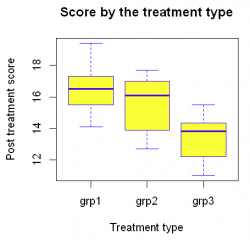
Based on the boxplot we can see that the anxiety mean score is the highest for individuals who have been practicing basal(grp1) type of exercises and the lowest for individuals who have been practicing the high(grp3) type of exercises. These observations are made based on descriptive statistic by not taking into consideration the overall personal ability of each individual to control his/her anxiety level, let us prove it statistically with the help of ANCOVA.
Checking assumptions
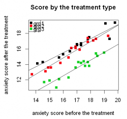
1. Linearity assumption can be assessed with the help of the regression fitted lines plot for each treatment group. Based on the plot bellow we can visually assess that the relationship between anxiety score before and after treatment is linear.
plot(x   = data$t1,
     y   = data$t3,
     col = data$group,
     main = "Score by the treatment type",
     pch = 15,
     xlab = "anxiety score before the treatment",
     ylab = "anxiety score after the treatment")

legend('topleft',
       legend = levels(data$group),
       col = 1:3,
       cex = 1,
       pch = 15)
abline(lm (t3[group == "grp1"]~ t1[group == "grp1"],
              data = data))
abline(lm (t3[group == "grp2"]~ t1[group == "grp2"],
              data = data))
abline(lm (t3[group == "grp3"]~ t1[group == "grp3"],
              data = data))
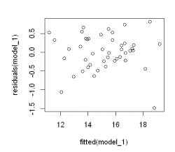
2. In order to evaluate whether the residuals are unbiased or not and whether the variance of the residuals is equal or not, a plot of residuals vs. dependent variable can be compiled. Based on the plot bellow we can conclude that the variances between the groups are homogeneous(homoscedastic). For interpretation of the plot please refer to this figure.
model_1 <- lm(t3~t1+group, data = data)

plot(fitted(model_1),
     residuals(model_1))
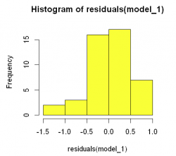
3. Homogeneity of residuals can be examined with the help of the Residual histogram and Shapiro-Wilk test.
hist(residuals(model_1),
     col="yellow")
#Shapiro-Wilk normality test
shapiro.test(residuals(model_1))
## Output:
## data:  residuals(model_1)
## W = 0.96124, p-value = 0.1362
Histogram of residual values is "bell shaped" and the Shapiro-Wilk normality test show p value of 0.1362 which is not significant (p>0.05) as a result we can concludevthat it is normally distributed.
4. Assumption of Homogeneity of regression slopes checks that there is no significant interaction between the covariate and the grouping variable. This can be assessed as follow:
options(contrasts = c("contr.treatment", "contr.poly"))

library(car)

model_2 <- lm(t3~t1+group+group:t1, data= data)
Anova(model_2, type = "II")
Interaction is not significant(p = 0.415), so the slope across the groups is not different.
Computation
When running the ANCOVA test in R attention should be paid on the orders of variables, because our main goal is to remove the effect of the covariate first. This notion is based on the general ANCOVA steps:
1) Run a regression between the independent(covariate) and dependent variables.
2) Identify the residual values from the results.
3) Run an ANOVA on the residuals.
Before running ANCOVA test with adjusted before treatment anxiety score (t1 = covariate) let us run the ANOVA test only on groups and after treatment anxiety score(t3) in order to see the impact of ANCOVA test on Sum of Squares of Errors.
model_3<- lm(t3~group, data = data)
Anova(model_3, type = "II")
model_1 <- lm(t3~t1+group, data = data)
Anova(model_1, type = "II")
As you can see after adjustment of berfore treatment anxiety score(t1 = covariate) Sum of Squares of Errors decreased from 102.83 to 9.47 meaning that the "noise" from covariate was taken under control by making it possible to evaluate the effect of treatment types only.
So let us recall our main question "What treatment type has the most effect on anxiety level?"
As we can see from the test result above there is a statistically significant difference in after treatment anxiety score between the groups, F(2, 41) = 218.63, p < 0.0001.
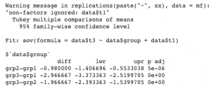
The F-test showed a significant effect somewhere among the groups. However, it did not tell us which pairwise comparisons are significant. This is where post-hoc tests come into play, which will hekp us to find out which groups differ significantly from one other and which do not. More formally, post-hoc tests allow for multiple pairwise comparisons without inflating the type I error.
anova_comp<-aov(data$t3~data$group+data$t1)
TukeyHSD(anova_comp,'data$group')
According to Tukey Post-Hoc test the mean anxiety score was statistically significantly greater in grp1 compared to the grp2 and grp3, which means that the treatment type 1 has the most effect on anxiety level.
What is two-way ANCOVA?
A two-way ANCOVA is, like a one-way ANCOVA, however, each sample is defined in two categorical groups. The two-way ANCOVA therefore examines the effect of two factors on a dependent variable – and also examines whether the two factors affect each other to influence the continuous variable.
