Difference between revisions of "Bootstrapping in Python"
| Line 90: | Line 90: | ||
===Example 2. Bootstrapping as an alternative to t-test (TO EDIT)=== | ===Example 2. Bootstrapping as an alternative to t-test (TO EDIT)=== | ||
| − | Bootstrap can be | + | Bootstrap can be implemented for analyzing difference between mean values of two samples. |
<syntaxhighlight lang="Python" line> | <syntaxhighlight lang="Python" line> | ||
| Line 117: | Line 117: | ||
</syntaxhighlight> | </syntaxhighlight> | ||
| − | + | Let us calculate the probability that we observe such a difference (1.63 in this case) only by chance. We will run bootstrap simulation as follows: | |
| − | 1. | + | 1. Randomly sample with replacement from each group separately.<br> |
| − | 2. Calculate the difference of means between | + | 2. Calculate the difference of means between two created samples.<br> |
| − | 3. | + | 3. Repeat n times. (We will choose n as num_samples = 1000 |
| + | 4. Visualize the resulted distribution of saved mean differences. | ||
| − | |||
| − | |||
<syntaxhighlight lang="Python" line> | <syntaxhighlight lang="Python" line> | ||
| − | |||
num_samples = 1000 | num_samples = 1000 | ||
| − | + | diffs = [] # list to save differences | |
| − | diffs = [] | ||
| − | |||
for i in range(num_samples): | for i in range(num_samples): | ||
| − | + | subsample_A = samples_A.sample(frac=1, replace=True) | |
| − | + | subsample_B = samples_B.sample(frac=1, replace=True) | |
| − | |||
| − | |||
| − | |||
# calculate difference of means of 2 subsamples | # calculate difference of means of 2 subsamples | ||
| Line 143: | Line 136: | ||
diffs.append(bootstrap_difference) | diffs.append(bootstrap_difference) | ||
| − | |||
| − | |||
| − | |||
| − | |||
| − | |||
| − | |||
| − | |||
| − | |||
| − | |||
| − | |||
| − | |||
| − | |||
| − | |||
| − | |||
| − | |||
| − | |||
| − | |||
</syntaxhighlight> | </syntaxhighlight> | ||
| − | + | This histogram represents the variability of the mean difference that could arise from sampling variations. | |
We can also visualize the bootstrap simulation for the difference of mean values: | We can also visualize the bootstrap simulation for the difference of mean values: | ||
Revision as of 13:50, 14 May 2024
THIS ARTICLE IS STILL IN EDITING MODE
Contents
Introduction
The term "bootstrap" is euphonic with the metaphor of pulling oneself up by one's bootstraps, signifying the achievement of the seemingly impossible without external assistance. Analogously, as seen in Raspe's tales of Baron Munchausen, who extricated himself and his horse from a swamp by his own hair, the Bootstrap technique enables the attainment of statistical insights independently, bypassing the need for predefined formulas.
Bootstrap is applicable for any samples. It is useful when:
1. observations are not described by normal distribution;
2. there are no statistical tests for the desired quantities.
Theoretical aspect
Bootstrapping (sometimes also just bootstrap) is a method for estimating statistical quantities without reliance on explicit formulas.
To derive a specified statistic for a sample (such as the mean or variance, quantile, etc.), using bootstrap, pseudo-samples or subsamples are generated from the original sample by drawing with replacement. The mean (variance, quantile, etc.) is then computed for each pseudo-sample. Theoretically, this process can be repeated multiple times, generating numerous instances of the parameter of interest and allowing for the assessment of its distribution.

Advantages:
1. Simplicity and flexibility.
2. No knowledge about data distribution is needed.
3. Helps to avoids the cost of repeating the experiment to get more data.
4. Usually provides a more accurate estimates of a statistic than "standard" methods utilizing normal distribution.
Disadvantages:
1. Computational intensity. The process involves resampling from the dataset multiple times, which might be time-consuming for extensive datasets.
2. Dependence on the original data. Bootstrapping assumes that the original dataset is representative of the population.
3. Sensitivity to outliers. Since bootstrap samples with replacement, outliers may be overrepresented in the resampled datasets, affecting the stability of the results.
Synthetic examples of bootstrapping
Example 1. Bootstrapping for quantile evaluation
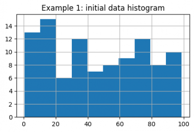
We will generate a sample with some random distribution:
import pandas as pd
import numpy as np
from scipy.stats import ttest_ind
import matplotlib.pyplot as plt

np.random.seed(42)

data = pd.Series(np.random.rand(100) * 100)

data.hist(figsize=(5, 3))
plt.title("Example 1: initial data histogram")
plt.show()
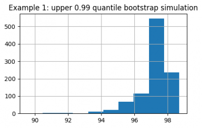
Using bootstrap to evaluate outliers in this case is much more reliable, than calculating normal distribution quantiles. For this purpose we will generate 1000 subsamples using pandas sample function and a loop. It is important to set replace=True, as bootstrap relies on drawing samples with replacement. We will evaluate the upper 0.99 and lower 0.01 quantiles.
upper_quantiles = []
lower_quantiles = []
for i in range(1000):
    subsample = data.sample(frac=1, replace=True)
    upper_quantiles.append(subsample.quantile(0.99))
    lower_quantiles.append(subsample.quantile(0.01))

upper_quantiles = pd.Series(upper_quantiles)
lower_quantiles = pd.Series(lower_quantiles)
We get an experimental distribution for both quantiles:
upper_quantiles.hist(figsize=(5, 3))
plt.title("Example 1: upper 0.99 quantile bootstrap simulation")
plt.show()
Now we can estimate confidence intervals for the upper and lower 0.01 quantiles:
# upper 0.99 quantile lies in this interval with 95% confidence
print(f'{upper_quantiles.quantile(0.025):.2f}') # Out: 94.89
print(f'{upper_quantiles.quantile(0.975):.2f}') # Out: 98.69

# lower 0.01 quantile lies in this interval with 95% confidence
print(f'{lower_quantiles.quantile(0.025):.2f}') # Out: 0.55
print(f'{lower_quantiles.quantile(0.975):.2f}') # Out: 4.62
Example 2. Bootstrapping as an alternative to t-test (TO EDIT)
Bootstrap can be implemented for analyzing difference between mean values of two samples.
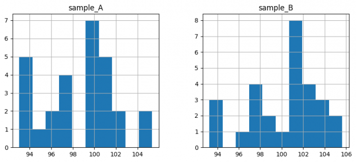
# generate 2 samples
samples_A = pd.Series(
    [100.24,  97.77,  95.56,  99.49, 101.4 , 105.35,  93.33,  93.02,
     101.37,  95.66,  93.34, 100.75, 104.93,  97.  ,  95.46, 100.03,
     102.34,  93.23,  97.05,  97.76,  93.63, 100.32,  99.51,  99.31,
     102.41, 100.69,  99.67, 100.99],
    name='sample_A')
samples_B = pd.Series(
    [101.67, 102.27,  97.01, 103.46, 100.76, 101.19,  99.11,  97.59,
     101.01, 101.45,  94.3 , 101.55,  96.33,  99.03, 102.33,  97.32,
      93.25,  97.17, 101.1 , 102.57, 104.59, 105.63,  93.93, 103.37,
     101.62, 100.62, 102.79, 104.19],
    name='sample_B')

pd.concat([samples_A, samples_B], axis=1).hist(figsize=(10, 4))
plt.show()
AB_difference = samples_B.mean() - samples_A.mean()
print(f"Difference of mean values {AB_difference:.2f}") # Out: Difference of mean values 1.63
Let us calculate the probability that we observe such a difference (1.63 in this case) only by chance. We will run bootstrap simulation as follows:
1. Randomly sample with replacement from each group separately.
2. Calculate the difference of means between two created samples.
3. Repeat n times. (We will choose n as num_samples = 1000
4. Visualize the resulted distribution of saved mean differences.
num_samples = 1000
diffs = [] # list to save differences

for i in range(num_samples):
    subsample_A = samples_A.sample(frac=1, replace=True)
    subsample_B = samples_B.sample(frac=1, replace=True)

    # calculate difference of means of 2 subsamples
    bootstrap_difference = subsample_B.mean() - subsample_A.mean()
    diffs.append(bootstrap_difference)
This histogram represents the variability of the mean difference that could arise from sampling variations.
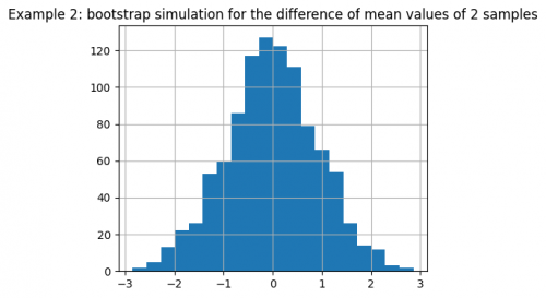
We can also visualize the bootstrap simulation for the difference of mean values:
pd.Series(diffs).hist(bins=20, figsize=(5, 4))
plt.title(
    "Example 2: bootstrap simulation for" +
    "the difference of mean values of 2 samples")
plt.show()
From the figure we conclude that value of 1.63 is quite rarely encountered in the simulation, making it unlikely that such a value for the initial samples is acquired by chance.
Compare this result to t-test:
ttest_ind(samples_A.values, samples_B.values)
# Out: TtestResult(statistic=-1.7971305016442471, pvalue=0.07790788332728987, df=54.0)Out: TtestResult(statistic=-1.7971305016442471, pvalue=0.07790788332728987, df=54.0)
The result is the similar, p-value is very small, the means differ significantly. However, t-test is much more "sure" about the results, while the p-value for bootstrapping was barely below threshold.
Further reading
1. https://medium.com/analytics-vidhya/what-is-bootstrapping-in-machine-learning-777fc44e222a (a simple article, also contains a link to the original article)
2. https://towardsdatascience.com/an-introduction-to-the-bootstrap-method-58bcb51b4d60 (a more mathematical article explaining why bootstrap actually works, has a lot of further links)
3. https://en.wikipedia.org/wiki/Bootstrapping_(statistics)
The author of this entry is Igor Kvachenok.


