Regression, Correlation, and Ordinary Least Squares Estimator in Python

THIS ARTICLE IS STILL IN EDITING MODE

Introduction

Regression analyses and assessment of correlation between different variables are common approaches when working with data in many different fields. Albeit it does not provide detailed insights into the mechanisms underlying the relationship of the variables investigated, it is a good first analysis to get an overview of what is going on. Correlation describes a linear relationship between at least two variables. It ranges between -1 and 1, which are called perfect positive and perfect negative correlation respectively. For example, a correlation between income (in Euros) and education (in years of schooling) of 0.5 indicates that there is a positive linear relationship between an increase in education and income. The most common approach to assessing corelation is via regression analysis. In regression analysis, a relationship between one dependent variable and at least on independent variable is assessed. With the help of the regression analysis, the effect of a change in the independent variable(s) by one unit on the dependent variable is modelled. This model therefore tries to find the linear curve that is best representing the actual relationship between the dependent and the independent variable(s). Returning to the example of income and education, we can set income to be the dependent variable and education as the independent variable. We can also add other variables affecting income, such as average wages in the country of the workplace (GDP), or relevant working experiences (in months of experience). With the regression analysis, we can then assess the change in income with a one unit increase of education and working experience, and an increase in GDP when having an international dataset. One of the most used estimators for assessing correlation is the ordinary least squares estimator (OLS). The OLS aims to produce a linear curve whose values minimize the sum of the squared values of the dependent variable and the predicted values from the regression equation. The OLS estimator relies on a number of assumptions that cannot be discussed in detail, but you can find them here. In the following, we will have a look at a record of computer science exercises results from students. We will prepare the data, do some analytic checks, and finally apply the OLS estimator.

Ordinary Least Squares Estimator

The following parameters are used:

id = final digit of the student matriculation number group = name of the learning group sex = gender in binary categories (m = male, f = female) quanti = number of solved exercises points = total score achieved from the exercises exam = total score achieved from the final written exam (Students must have to participate in the final written exam. If not, they will be considered as fail) passed = dummy whether the person has passed the class or not

Firstly, the aim for analyzing the dataset is to figure out the performance scored among the learning groups and gender for the solved questions, exercises and written exams.

Secondly, we want to figure out the correlation between variables and most importantly to figure out heteroscedastic and homoscedastic dispersion, since the OLS is only apt when homoscedasticity is the case.

To analyse this data, some python libraries have to be imported:

import pandas as pd ## to organize data
import numpy as np ## to make mathematical computations
import statsmodels.api as sm ## needed for statistial anaysis
import statsmodels.formula.api as smf ## needed to write more complex statistical models
import matplotlib.pyplot as plt ## to make plots
import seaborn as sns ## for visualization
from statsmodels.formula.api import ols ## to use OLS
from sklearn import preprocessing ## needed for regression analysis
from statsmodels.stats.diagnostic import het_breuschpagan ## for checking your multiple regression model

Data Inspection

Data inspection is made to check if the data is clean for better graphical performance. The cleaning involves checking for missing values and the data format. The dataset is randomly generated based on a few cornerstone observations from an actual data science class. You can find the data here.

data = pd.read_csv('final.csv')

data.head(16)## looks at the first 16 rows

data.tail(16)## looks at the last 16 rows

data.isnull().sum()## checks if there is missing data

bool_series = pd.isnull(data['exam'])## Assesses if the exam value takes 0 or not in Boolean terms (exam is 0 = TRUE, exam not 0 = FALSE).
(data[bool_series])#Chooses only the rows where the exam is 0 (NaN)

len(data[bool_series])#applying the bool series by checking the null value

data = data.dropna()
data #now, only the rows without the Nas are part of the dataset

data.shape# you can see here the number of rows (72) and columns (7)

Result: (72,7)

duplicates= data.duplicated()## checks for duplicates which would distort the results
print(duplicates)

There is no duplicated data so we can move on analyising the dataset.

data.info()

Here, you can get an overview over the different datatypes, if there are missing values ("non-null") and how many entries each column has. Our columns where we wish to make a quantitative analysis should be int64 (without decimal components) or float64 (with decimal components), but id can be ignored since it is only an individual signifier. The variables with the "object" data format can contain several data formats. However, looking at the three variables, we can see that they are in a categorical data format, having the categories for gender, whether one passed an exam or not, and the category of the different study groups. These categorical variables cannot be used for a regression analysis as the other variables since we cannot analyze an increase in one unit of this variables and its effect on the dependent variable. Instead, we can see how belonging to one of the categories affects the independent variable. For "sex" and "passed", these are dummy variables. Columns we will treat as dummy variables can take categories in binary format. We can then for example see if and how being female impacts the dependent variable.

data.describe()## here you can an overview over the standard descriptive data.

data.columns #This command shows you the variables you will be able to use. The data type is object, since it contains different data formats.

Homoscedasticity and Heteroscedasticity

Before conducting a regression analysis, it is important to look at the variance of the residuals. In this case, the term ‘residual’ refers to the difference between observed and predicted data (Dheeraja V.2022).

If the variance of the residuals is equally distributed, it is called homoscedasticity. Unequal variance in residuals causes heteroscedastic dispersion.

If heteroscedasticity is the case, the OLS is not the most efficient estimating approach anymore. This does not mean that your results are biased, it only means that another approach can create a linear regression that more adequately models the actual trend in the data. In most cases, you can transform the data in a way that the OLS mechanics function again. To find out if either homoscedasticity or heteroscedasticity is the case, we can look at the data with the help of different visualization approaches.

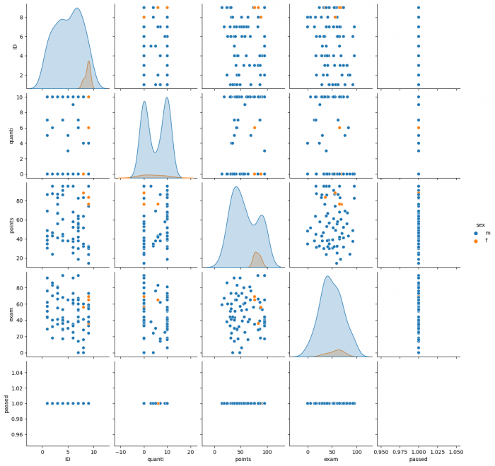
sns.pairplot(data, hue="sex") ## creates a pairplot with a matrix of each variable on the y- and x-axis, but gender, which is colored in orange (hue= "sex")

The pair plot model shows the overall performance scored of the final written exam, exercise and number of solved questions among males and females (gender group).

Looking a the graphs along the diagonal line, it shows a higher peak among the male students than the female students for the written exam, solved question (quanti) and exercise points (points). Looking at the relationship between exam and points, no clear pattern can be identified. Therefore, it cannot be safely assumed, that a heteroscedastic dispersion is given.

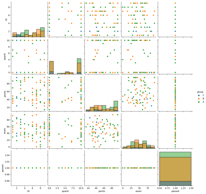
sns.pairplot(data, hue="group", diag_kind="hist")

The pair plot model shows the overall performance scored in the final written exam, for the exercises and number of solved questions solved among the learning groups A,B and C.

The histograms among the diagonal line from top left to bottom right show no normal distribution. The histogram for id can be ignored since it does not provide any information about the student records. Looking at the relationship between exam and points, a slight pattern could be identified that would hint to heteroscedastic dispersion.

Correlations with Heatmap

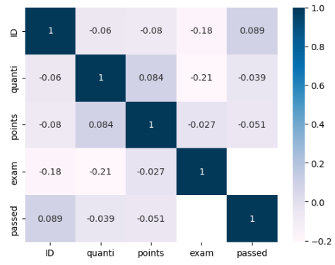
A heatmap shows the correlation between different variables. Along the diagonal line from left to right, there is perfect positive correlation because it is the correlation of one variable against itself. Generally, you can assess the heatmap fully visually, since the darker the square, the stronger the correlation.

p=sns.heatmap(data.corr(),
              annot=True, cmap='PuBu');

The results of the heatmap are quite surprising. There is no positive correlation between any activity prior to the exam and the exam points scored. In fact, a negative correlation between quanti and exam of -0.21 is considerably large. If this is confirmed in the OLS, one explanation could be that the students lacked time to study for the exam because of the number of exercises solved. The only positive, albeit not too strong correlation can be found between points and quanti. This positive relationship seems intuitive considering that with an increased number of exercises solved, the total of points that can be achieved increases and the students will generally have more total points.

OLS

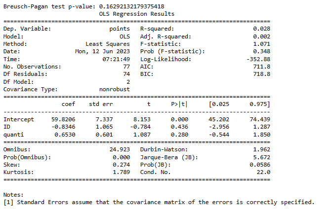
Now, we will have a look at different OLS approaches. We will test for heteroscedasticity formally in each model with the Breusch-Pagan test.

model_1 = smf.ols(formula='points ~ ID + quanti', data=data) ## defines the first model with points being the dependent and id and quanti being the independendet variable
result_bp1 = model_1.fit()

# Checking for heteroscedasticity using the Breusch-Pagan test
bp1_test = het_breuschpagan(result_bp1.resid, result_bp1.model.exog)

# Print the Breusch-Pagan test p-value
print("Breusch-Pagan test p-value:", bp1_test[1])

## If the p value is smaller then the set limit (e.g., 0.05, we need to reject the assumption of homoscedasticity and assume heteroscedasticity).

result = model_1.fit() ## estimates the regression

print(result.summary()) ## print the result

Looking at the Breusch-Pagan test, we can see that we cannot reject the assumption of homoscedasticity. Considering the correlation coefficients, no statistically significant relationship can be identified. The positive relationship between quanti and points can be found again, but it is not statistically significant.

import statsmodels.formula.api as smf
from statsmodels.stats.diagnostic import het_breuschpagan

model_2 = smf.ols(formula='points ~ ID + sex', data=data)
result_bp2 = model_2.fit()

# Checking for heteroscedasticity using the Breusch-Pagan test
bp2_test = het_breuschpagan(result_bp2.resid, result_bp2.model.exog)

# Print the Breusch-Pagan test p-value
print("Breusch-Pagan test p-value:", bp2_test[1])

# Set the value for maxlags
maxlags = 25  # Update this value as needed

result = model_2.fit(cov_type='HAC', cov_kwds={'maxlags': maxlags})
print(result.summary())

# Assuming 'sex' is a column in the DataFrame named 'data'
sex_counts = data['sex'].value_counts()

# Print the frequency table
print(sex_counts)

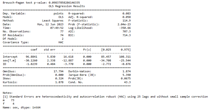
Based on the Breusch-Pagan test, the assumption of homoscedasticity needs to be rejected to the 0.1% significance level. Therefore, we correct for heteroscedasticity with HAC (for more details see here) Looking at the results, being female ("sex") has a large negative effect on points and is highly statistically significant. However, looking at the number of females in the dataset, we need to be very cautious to draw any conclusions. Since there are only four females in the dataset (and 73 males), the sample size is considered too small to make any statements about gendered effects on total points achieved. The correlation between ID and points can be ignored, since the last number of the matricle numbers follow no pattern.

import statsmodels.formula.api as smf
from statsmodels.stats.diagnostic import het_breuschpagan

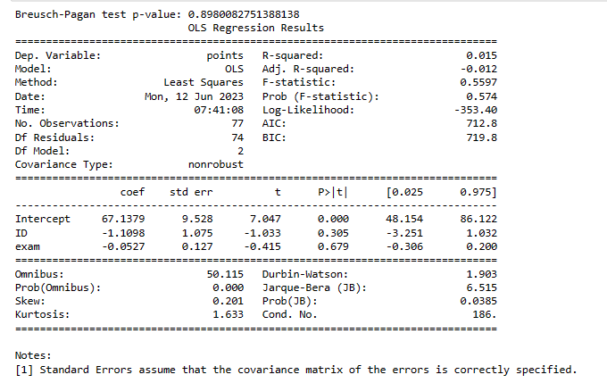
model_3 = smf.ols(formula='points ~ ID + exam', data=data)
result_bp2 = model_3.fit()

# Checking for heteroscedasticity using the Breusch-Pagan test
bp2_test = het_breuschpagan(result_bp3.resid, result_bp3.model.exog)

# Print the Breusch-Pagan test p-value
print("Breusch-Pagan test p-value:", bp3_test[1])

result = model_3.fit()
print(result.summary())

Based on the Breusch-Pagan test, the asssumption of homoscedasticity cannot be rejected to the 0.1% significance level. Looking at the results, no statistically significant result can be found, albeit the slight neative relationship between exam and points can also be found in the OLS.

Conclusion

There are many steps needed, before a regression analysis can be conducted. First, the data needs to be prepared, for example the Nas need to be removed. Then, the data needs to be assessed visually, to gain an understanding of potential homo- or heteroscedasticity. Finally, after testing for heteroscedasticity, the regression can be run, albeit the results always need to be considered in light of the available data, such as with the case for the effect of gender on total points achieved.

References

1.Iqbal H.(2020),Linear Regression Analysis, Source:https://www.kaggle.com/datasets/iqbalrony/linear-regression-analysis , Accessed: 20.12.2022

2.Dheeraja V.(2022),Heteroskedasticity,Source :https://www.wallstreetmojo.com/heteroskedasticity/ ,Accessed:20.12.2022

3.Econometrics(2022),Introduction to Econometrics with R ,Source :https://www.econometrics-with-r.org/5-4-hah.html , Accessed view:24.12.2022

The author of this entry is XX. Edited by Milan Maushart.