Permutation Test
THIS ARTICLE IS STILL IN EDITING MODE
Contents
Introduction
Permutation testing, a non-parametric statistical method, offers a robust alternative to traditional hypothesis testing. It is particularly useful in scenarios where the assumptions required for parametric tests are not met. By reshuffling the data and observing the outcomes, permutation tests provide an empirical approach to hypothesis testing, making them adaptable to a wide range of data types and distributions. Imagine you have a bunch of data points, and you are trying to find out, if there is a meaningful pattern or just random noise. Permutation testing helps with this by mixing up the data and looking at what happens. It is similar to shuffling a deck of cards to see, if a particular arrangement happens just by chance.
Think of permutation testing as a cousin to another method called 'bootstrap'. Both use random shuffling of your data, but they have different goals. Bootstrap is about understanding how your sample represents a bigger population. In contrast, permutation testing is more about playing the 'what-if' game: what if there was no specific pattern in the data? It tries to see, what kind of random patterns can pop up when there is actually no real structure in the data. In other words, permutation is best for testing hypotheses and bootstrap is best for estimating confidence intervals.
Concept of Permutation Testing
At the heart of permutation testing is a simple question: Are different groups really different in terms of some statistical measure, or is it just a coincidence? To answer this, we start with the assumption (called the null hypothesis) that there is no difference between the groups.
Here is how it works: for instance, you have groups A and B (and maybe C, D, and so on). You mix all their data points together because, according to your starting assumption, they are all the same. This mixing represents the idea that the specific treatment or condition each group experienced does not really make a difference. Then you create new groups from this big mixed pool of data and calculate your statistic (like an average) for these new groups. By doing this over and over and seeing how much these new groups differ from each other, you can start to understand, if the original difference between A and B was real or just a coincidence.
Steps in Permutation Testing in Python
1. Combining Data: Data from different groups are combined, embodying the null hypothesis of no significant difference.
2. Resampling: The combined data is repeatedly shuffled, and resamples are drawn to mimic the original sample sizes.
3. Calculating Statistics: For each permutation, the statistic of interest (e.g., mean difference) is calculated.
4. Forming Distribution: This process is repeated numerous times, generating a distribution of the test statistic under the null hypothesis.
5. Comparison and Conclusion: The actual test statistic calculated from the original data is compared with this distribution. If it lies in the extreme, the null hypothesis is rejected, indicating statistical significance.
#Create Dataset
import pandas as pd
import numpy as np
import matplotlib.pyplot as plt

# Define the sample size for each group
sample_size_a = 1000
sample_size_b = 700

# Generate random data for each group
# Assuming a normal distribution for both groups with the same mean and standard deviation
np.random.seed(42)

# Generate data for two groups with different sample sizes
group_a = np.random.normal(loc=50, scale=10, size=30)  # Group A with 30 samples
group_b = np.random.normal(loc=55, scale=15, size=40)  # Group B with 40 samples

# Create a DataFrame
df = pd.DataFrame({
    "Group": ["A"]*30 + ["B"]*40,
    "Value": np.concatenate([group_a, group_b])
})

df.head()
| Group | Value | |
|---|---|---|
| 0 | A | 54.967142 |
| 1 | A | 48.617357 |
| 2 | A | 56.476885 |
| 3 | A | 65.230299 |
| 4 | A | 47.658466 |
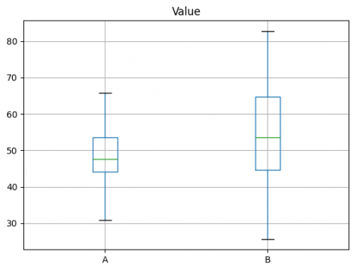
ax = df.boxplot(by='Group', column='Value')
ax.set_xlabel('')
plt.suptitle('')
mean_a = df[df.Group == 'A'].Value.mean()
mean_b = df[df.Group == 'B'].Value.mean()
abs(mean_b - mean_a)
5.461927449669801
Group B has Value that are greater than those of A by 5.4 on average. The question is whether this difference is within the range of what random chance might produce, i.e., is statistically significant. One way to answer this is to apply a permutation test — combine all the session times together and then repeatedly shuffle and divide them into groups of 30 and 40 (recall that nA = 30 for Group A, and nB = 40 for Group B).
To apply a permutation test, we need a function to randomly assign the 70 samples to a group of 30 (Group A) and a group of 40 (Group B).
#Create Permutation Function
import random
def perm_fun(x, nA, nB):
 n = nA + nB
 idx_B = set(random.sample(range(n), nB))
 idx_A = set(range(n)) - idx_B
 return x.loc[idx_B].mean() - x.loc[idx_A].mean()

nA = df[df.Group == 'A'].shape[0]
nB = df[df.Group == 'B'].shape[0]
print(perm_fun(df.Value, nA, nB))
-1.334223479417716
This function works by sampling (without replacement) nB indices and assigning
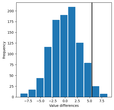
them to the B group; the remaining nA indices are assigned to group A. The difference between the two means is returned. Calling this function R = 1000 times and specifying nA = 30 and nB = 40 leads to a distribution of differences in the session times that can be plotted as a histogram. In Python this is done as follows using the hist() method:
perm_diffs = [perm_fun(df.Value, nA, nB) for _ in range(1000)]

fig, ax = plt.subplots(figsize=(5, 5))
ax.hist(perm_diffs, bins=11, rwidth=0.9)
ax.axvline(x = mean_b - mean_a, color='black', lw=2)
ax.set_xlabel('Value differences')
ax.set_ylabel('Frequency')
np.mean(perm_diffs > mean_b - mean_a)
0.031
In the context of a permutation test, this value is the empirical p-value for the test. This suggests that the observed difference in Value between Group A and Group B is not within the range of chance variation and thus is statistically significant difference from each others.
Strengths & Challenges
Strengths
- Good for exploring the role of random variation.
- Relatively easy to code, interpret, and explain.
- Data can be numeric or binary.
- Sample sizes can be the same or different
- Does not require normally distributed data
- Does not require large sample size.
Challenges
- Computationially Expensive
- Assume that observations are exchangeable under the null hypothesis. If this assumption is violated, for example, in time series data where observations are correlated, the test may not be valid.
- Assume that the null hypothesis involves some form of equality (e.g., equal means). They are not designed to test more complex null hypotheses without adaptation.
References
1. Edgington, E., & Onghena, P. (2007). Randomization Tests (4th ed.). Chapman & Hall/CRC Press.
2. Bruce, P. (2014). Introductory Statistics and Analytics: A Resampling Perspective. Wiley.
3. Bruce, P., & Bruce, A. (2017). Practical Statistics for Data Scientists. O'Reilly Media, Inc. ISBN 9781491952962.
The author of this entry is Matthew Eiampikul.

