Field experiments

Note: This entry revolves mostly around field experiments. For more details on experiments, please refer to the entries on Experiments and Hypothesis Testing, Case studies and Natural experiments as well as Experiments.

The field experiment

Field experiments were as you may could guess first conducted in agriculture.

With a rise in knowledge, it became apparent that the controlled setting of a laboratory was not enough. First in astronomy, but then also in agriculture and other fields the notion became apparent that our reproducible settings may sometimes be hard to achieve. Observations can be unreliable, and error of measurements in astronomy was a prevalent problem in the 18th and 19th century. Fisher equally recognised the mess - or variance - that nature forces onto a systematic experimenter. The demand for more food due to the rise in population, and the availability of potent seed varieties and fertiliser - both made possible thanks to scientific experimentation - raised the question how to conduct experiments under field conditions. Making experiments in the laboratory reached its outer borders, as plant growth experiments were hard to conduct in the small confined spaces of a laboratory, and it was questioned whether the results were actually applicable in the real world. Hence experiments literally shifted into fields, with a dramatic effect on their design, conduct and outcome. While laboratory conditions aimed to minimise variance - ideally conducting experiments with a high confidence -, the new field experiments increased sample size to tame the variability - or messiness - of factors that could not be controlled, such as subtle changes in the soil or microclimate. Establishing the field experiment became thus a step in the scientific development, but also in the industrial development. Science contributed directly to the efficiency of production, for better or worse.

Key concepts in the application of field experiments

The arbitrary p value

You are probably already familiar with this type of overview but it is one of the most commen research designs.

The analyis of variance was actually inspired widely by field experiments, as Fisher was working with crop data which proved as a valuable playground to develop and test his statistical approaches. It is remarkable that the p-value was actually chosen by him and did not follow any wider thinking within a community. Probably not since Linne or Darwin did a whole century of researchers commit their merits to a principle derived by one person, as scientific success and whole careers are build on results measured by the p-value. It should however be noted that the work needed to generate enough replicates to measure probability with Fishers measure of 0.05 was actually severe within crop experiments when compared to lab settings. In a lab you can have a few hundred Petri dishes or plant pots and these can be checked by a lab technician. Replicates in an agricultural field are more space and labour intense, while of course lab space is more expensive per square meter. In order to design field experiments where enough replicates were made, in order to enable testing at an appropriate significance level, demanded nothing less than a revolution in the planning of studies. With all its imperfections and criticism, Fishers use of the p-value can probably be credited for increasing sample number in experiments towards a sensible and sufficient level. Study designs became the new norm, and are an essential part of science ever since.

Randomisation

Field experiments are often divided into quadrangles, and these then represent a certain treatment or treatment combination. In a randomized experiment, a study sample is then randomly divided into treatment and control groups.

Field experiments try to compensate for gradients that infer variance within a sample design by increasing the number of samples. However, in order to uncouple the effects of underlying variance, randomisation is central. Take the example of an agricultural field that has more sandy soils on one end, and more loamy soils on the other end. If now all samples of one treatment would be on the loamy end of the field, and all samples of another treatment would be at the sandy end of the field, then the treatment effect would contain an artefact of the soil gradient. Randomisation in fields is hence essential to maximize independence of the treatment effect from the underlying variance. A classical chessboard illustrates the design step of randomisation quite nicely, since field experiments are often divided into quadrangles, and these then represent a certain treatment or treatment combination. Especially in agricultural fields, such an approach was also following a certain pragmatism, since neighbouring quadrangles might have a tendency to influence each other, i.e. through root competition. While this error is often hard to take into account, it is quite relevant to notice that enough replicates might at least allow to tame this problem, and make the error introduced by such interactions less relevant overall. Just as we should apply randomisation when sampling for instance a representative sample from a population, the same approach is applied in the design of experiments.

Blocking

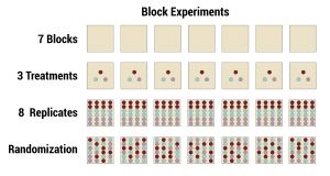
Designing an experiment using block effects.

In order to tame the variance of the real world, blocking was a plausible approach. By basically introducing agricultural fields as blocks, the variance from individual blocks can be tamed. This was one of the breakthroughs, as the question of what we want to know i.e. hypothesis testing, was statistically uncoupled from the question what we do not want to know, i.e. the variance inferred from individual blocks. Consequently, the samples and treatment combinations need to be randomised within the different blocks, or can be alternatively replicated within these blocks. This has become established as a standard approach in the designing of experiments, often for rather pragmatic reasons. For instance are agricultural fields often showing local characteristics in terms of soil and microclimate, and these should be tamed by the clear designation of blocks and enough blocks in total within the experiment. The last point is central when thinking in terms of variance, since it would naturally be very hard to think in terms of variance regarding e.g. only two blocks. A higher number of blocks allow to better tame the block effect. This underlines the effort that often needs to go into designing experiments, since a sufficient number of blocks would basically mean that the effort can be multiplied by the number of blocks that are part of the design. Ten blocks means ten times as much work, and maybe with the result that there is no variance among the blocks overall.

Nested designs

A nested design is used for experiments in which there is an interest in a set of treatments and the experimental units are sub-sampled.

Within field experiments, one factor is often nested within another factor. The principle of nestedness works generally like the principle of Russian dolls: Smaller ones are encapsulated within larger ones. For instance can a block be seen as the largest Russian doll, and the treatments are then nested in the block, meaning each treatment is encapsulated within each block. This allows for a testing where the variance of the block effect can be minimised, and the variance of the treatment levels can be statistically compared. Quite often the variance across different levels of nestedness is a relevant information in itself, meaning for instance how much variance is explained by a different factor. Especially spatially nested designs can have such a hierarchical structure, such as neighbourhoods within cities, streets within neighbourhoods and houses in streets. The nested structure would in this case be Cities/neighbourhoods/streets/houses. Just as with blocks, a nested structure demands a clear designing of an experiment, and greatly increase the sample size. Hence such a design should be implemented after much reflection, based on experience, and ideally by consultation with experts both in statistics as well as the given system.

Analysis

How to grow our plants best? If we simplify our model and eliminate nonsignificant treatments, we may find out.

The analysis of field experiments demands great care, since this is mostly a deductive approach where equal emphasis is put on what we understand, and what we do not understand. Alternatively, we could highlight that rejection of the hypothesis is the most vital step of any experiment. In statistical terms the question of explained vs. unexplained variance is essential. The first step is however checking the p-value. Which treatments are significant, and which ones are not? When it comes to two-way ANOVAs, we may need to reduce the model to obtain a minimum adequate model. This basically equals a reduction of the full model into the most parsimonious version, following Occam's razor. While some researchers tend to report the full model, with all non-significant treatments and treatment combinations, I think this is wrong. If we reduce the model, the p-values change. This can make the difference between a treatment that is significant, and a non-significant model. Therefore, model reduction is being advised for. For the sake of simplicity, this can be done by first reducing the highest level interactions that are not significant. However, the single effects always need to be included, as the single effects are demanded if interactions of a treatment are part of the model, even if these single effects are not significant. An example of such a procedure would be the NPK dataset in R - it contains information about the effect of nitrogen, phosphate and potassium on the growth of peas. There, a full model can be constructed, and then the non-significant treatments and treatment interactions are subsequently removed to arrive at the minimum adequate model, which is the most parsimonious model. This illustrates that Occam's razor is not only a theoretical principle, but has direct application in statistics.

#the dataset npk contains information about the effect of nitrogen, phosphate and potassium on the growth of peas
#let us do a model with it
data(npk)
str(npk)
summary(npk)
hist(npk$yield)

par(mfrow=c(2,2))
par(mar=c(2,2,1,1))
boxplot(npk$yield~npk$N)
boxplot(npk$yield~npk$P)
boxplot(npk$yield~npk$K)
boxplot(npk$yield~npk$block)
graphics.off()

mp<-boxplot(npk$yield~npk$N*npk$P*npk$K)#tricky labels
#we can construct a full model
model<-aov(yield~N*P*K,data=npk)
summary(model)

#then the non-significant treatments and treatment interactions are subsequently removed 
#to arrive at the minimum adequate model
model2<-aov(yield~N*P*K+Error(block),data=npk)
summary(model2)

model3<-aov(yield~N+P+K+N:P+N:K+P:K+Error(block),data=npk)
summary(model3)

model4<-aov(yield~N+P+K+N:P+N:K+Error(block),data=npk)
summary(model4)

model5<-aov(yield~N+P+K+N:P+Error(block),data=npk)
summary(model5)

model6<-aov(yield~N+P+K+Error(block),data=npk)
summary(model6)

model7<-aov(yield~N+K+Error(block),data=npk)
summary(model7)

Once we have a minimum adequate model, we might want to check the explained variance as well as the unexplained variance. Within a block experiment we may want to check how much variance is explained on a block level. In a nested experiment, the explained variance among all levels should be preferably checked. In a last step, it could be beneficial to check the residuals across all factor levels. While this is often hampered by a smaller sample size, it might be helpful to understand the behaviour of the model, especially when initial inspection in a boxplot showed flaws or skews in the distribution.

Fixed effects vs. Random effects

If smoking is a fixed or a random effect depends on the study design

Within ANOVA designs, the question whether a variable is a fixed or a random factor is often difficult to consider. Generally, fixed effects are about what we want to find out, while random effects are about aspects which variance we explicitly want to ignore, or better, get rid of. However, it is our choice and part of our design whether a factor is random or fixed. Within most medical trials the information whether someone smokes or not is a random factor, since it is known that smoking influences much of what these studies might be focusing about. This is of course different if these studies focus explicitly on the effects of smoking. Then smoking would be a fixed factor, and the fact whether someone smokes or not is part of the research. Typically, factors that are part of a block design are random factors, and variables that are constructs relating to our hypothesis are fixed variables. To this end, it is helpful to consult existing studies to differentiate between random and fixed factors. Current medical trials may consider many variables, and have to take even more random factors into account. Testing the impact of random factors on the raw data is often a first step when looking at initial data, yet this does not help if it is a purely deductive design. In this case, simplified pre-tests are often a first step to make initial attempts to understand the system and also check whether variables - both fixed or random - are feasible and can be utilised in the respective design. Initial pre-tests at such smaller scales are a typical approach in medical research, yet other branches of research reject them as being too unsystematic. Fisher himself championed small sample designs, and we would encourage pre-tests in field experiments if at all possible. Later flaws and errors in the design can be prevented, although form a statistical standpoint the value of such pre-tests may be limited at best.

Unexplained variance

Karl Popper emphasised that facts can only be approximated, i.e. are only considered to be true as long as they are not falsified.

Fisher's approach of considering the variance of the real world in statistics can be seen as perfectly complementary to Popper's epistemological reflections.

Acknowledging unexplained variance was a breakthrough in modern science, as we should acknowledge that understanding a phenomena fairly well now is better than understanding something perfectly, but never. In a sense was the statistical developing of uncertainty reflected in philosophical theory, as Karl Popper highlighted the imperfection of experiments in testing or falsification of theories. Understanding the limitations of the scientific endeavour thus became an important baseline, and the scientific experiments tried partly to take this into account through recognising the limitations of the result. What is however often confused is whether the theory is basically imperfect - hence the results are invalid or implausible - or whether the experiment was conducted in an imperfect sense, making the results unreliable. The imperfection to understand the difference between flaws in theory and flaws in conducting the experiment is a continuous challenge of modern science. When looking at unexplained variance, we always have to consider that our knowledge can be limited through theory and empirical conduct, and these two flaws are not clearly separated. Consequently, unexplained variance remains a blank in our knowledge, and should always be highlighted as such. As much as it is important to acknowledge what we know, it is at least equally important to highlight what we do not know.

Interpretation of field experiments

Interpreting results from field experiments demands experience. First of all, we shall interpret the p-value, and check which treatments and interactions are significant. Here, many researchers argue that we should report the full model, yet I would disagree. P-values in ANOVA summaries differ between the so called full models -which include all predictors- and minimum adequate models -which thrive to be the most parsimonious models. Model reduction is essential, as the changing p-values may make a difference between models that are reporting true results, or flawed probabilities that vaporize once the non-significant terms are subsequently reduced. Therefore, one by one we need to minimize the model in its complexity, and reduce the model until it only contains significant interaction terms as well as the maybe even non-significant single terms, which we have to include if the interaction is significant. This will give us a clear idea which treatments have a significant effect on the dependent variable. Second, when expecting model results we should interpret the sum of squares, thereby evaluating how much of the respective treatment is explain the effect of the dependent variable. While this is partly related to the p-value, it is also important to note how much variance is explained by potential block factors. In addition, it is also important to notice how much remains unexplained in total, as this residual variance indicates how much we do not understand using this experimental approach. This is extremely related to the specific context, and we need to be aware that knowledge of previous studies may aid us in understanding the value of our contribution. Lastly, we need to take further flaws into our considerations when interpreting results from field experiments. Are there extreme outliers. How do the residuals look like? Is any treatment level showing signs of an uneven distribution or gaps? Do the results seem to be representative? We need to be very critical of our own results, and always consider that the results reflect only a part of reality.

Replication of experiments

One famous example from the discipline of psychology is the Milgram shock experiment carried out by Stanley Milgram a professor from the Yale University in 1963.

Field experiments became a revolution for many scientific fields. The systematic testing of hypotheses allowed first for agriculture and other fields of production to thrive, but then also did medicine, psychology, ecology and even economics use experimental approaches to test specific questions. This systematic generation of knowledge triggered a revolution in science, as knowledge became subsequently more specific and detailed. Take antibiotics, where a wide array of remedies was successively developed and tested. This triggered the cascading effects of antibiotic resistance, demanding new and updated versions to keep track with the bacteria that are likewise constantly evolving. This showcases that while the field experiment led to many positive developments, it also created ripples that are hard to anticipate. There is an overall crisis in complex experiments that is called replication crisis. What is basically meant by that is that some possibilities to replicate the results of studies -often also of landmark papers- failed spectacularly. In other words, a substantial proportion of modern research cannot be reproduced. This crisis affects many arenas in sciences, among them psychology, medicine, and economics. While much can be said about the roots and reasons of this crisis, let us look at it from a statistical standpoint. First of all, at a threshold of p=0.05, a certain arbitrary amount of models can be expected to be significant purely by chance. Second, studies are often flawed through the connection between theory and methodological design, where for instance much of the dull results remains unpublished, and statistical designs can biased towards a specific results. Third, statistics slowly eroded into a culture where more complex models and the rate of statistical fishing increased. Here, a preregistration of your design can help, which is often done now in psychology and medicine. Researchers submit their study design to an external platform before they conduct their study, thereby safeguarding from later manipulation. Much can be said to this end, and we are only starting to explore this possibility in other arenas. However, we need to be aware that also when we add complexity to our research designs, especially in field experiments the possibility of replication diminished, since we may not take factors into account that we are unaware of. In other words, we sacrifice robustness with our ever increasing wish for more complicated designs in statistics. Our ambition in modern research thus came with a price, and a clear documentation is one antidote how we might cure the flaws we introduced through our ever more complicated experiments. Consider Occam’s razor also when designing a study.