Data Inspection in Python

THIS ARTICLE IS STILL IN EDITING MODE

Pretext

Data inspection is an important and necessary step in data science because it allows data scientists to understand the characteristics of their data and identify potential problems or issues with it. By carefully inspecting the data, data scientists can ensure that the data is accurate, complete, and most importantly relevant to the problem they are trying to solve.

Where to find Data?

There are many platforms where you can find data. These are five common and reliable ones:

Let's Start the Data Inspection

For our data inspection, we will be using the following packages: 1. Pandas, which is a standard data analysis package, and 2. Matplotlib, which can help us create beautiful visualizations of our data. We can import the packages as follows:

import pandas as pd
import matplotlib.pyplot as plt
# shows more columns
pd.set_option('display.max_columns', 500)

Load the data

To load the data, we need to use the appropriate command depending on the type of data file we have. For example, if we have a CSV file, we can load it using the read_csv method from Pandas, like this:

# data source: https://www.kaggle.com/datasets/ssarkar445/crime-data-los-angeles?resource=download
# downloaded 25.11.2022
# load data
data = pd.read_csv("Los_Angeles_Crime.csv")

If we have an Excel file, we can load it using the read_excel method, like this:

data = pd.read_excel("data_name.xlsx") #excel file

For more information about how to load different types of data files using Pandas, you can check out the pandas documentation (https://pandas.pydata.org/pandas-docs/stable/user_guide/io.html) (https://pandas.pydata.org/pandas-docs/stable/user_guide/io.html (https://pandas.pydata.org/pandas-docs/stable/user_guide/io.html)).

Size of Data

We check the size of the data by using the shape method, like this:

num_rows, num_cols = data.shape
print('The data has {} rows and {} columns'.format(num_rows, num_cols))

The data has 407199 rows and 28 columns.

The first number is the number of rows (data entries). The second number is the number of columns (attributes). Knowing the number of rows and columns in the data can be useful for a few reasons. First, it can help you make sure that the data has been loaded correctly and that you have the expected number of rows and columns. This can be especially important when working with large datasets, as it can be easy to accidentally omit or include extra rows or columns.

Basic info about data

To get basic information about the data, we can use the info method from Pandas, like this:

print(data.info())

This will print out a range of information about the data, including the number of entries and columns, the data types of each column, and the number of non- null entries. This information is useful for understanding the general structure of the data and for identifying potential issues or inconsistencies that need to be addressed. The following information is then shown:

RangeIndex: number of data entries
Data columns: number of columns
Table with
#: Column Index
Column: Column Name
Non-Null Count: number of non-null entries
Dtype: datatype (int64 and float64 are numerical, object is a string)

Knowing the data types of each column is important because different types of data require different types of analysis and modeling. For example, numeric data (e.g. numbers) can be used in mathematical calculations, while categorical data (e.g. words or labels) can be used in classification models. The following table shows all important data types.

Pandas Data Type	Python Data Type	Purpose
object	string	text/characters
int64	int	integer
float64	float	Decimal numbers
bool	bool	True or False
category	not available	Categorical data
datetime64	not avaiable	Date and time

Table Source The data types can also be specifically called upon using the dtypes method:

#types of data
print(data.dtypes)

First look at data

To get a first look at the data, we can use the head and tail methods from Pandas, like this:

# shows first and last five rows
print(data.head())
print(data.tail())

The head method will print the first few rows of the data, while the tail method will print the last few rows. This is a common way to quickly get an idea of the data and make sure that it has been loaded correctly. When working with large datasets, it is often not practical to print the entire dataset, so printing the first and last few rows can give you a general sense of the data without having to view all of it. Also, looking at the actual data helps us find out what type of data we are dealing with. Tip: Check out the documentation of the data source. In this case in kaggle about the "Crime Data Los Angeles", one can find some explanations about the columns.

Statistical info about data: To get a descriptive statistical overview of the data, we can use the described method from Pandas, like this:

print(data.describe())

This will calculate basic statistics for numeric columns, such as the mean, standard deviation, minimum and maximum values, and other summary statistics. This can be a useful way to get a general idea of the data and identify potential issues or trends. The output of the described method will be a table with the following attributes:

count: the number of non-null entries
mean: the mean value
std: the standard deviation
min: the minimum value
25%, 505, 75%: the lower, median, and upper quartiles
max: the maximum value

Check for missing values To check if the data has any missing values, we can use the isnull and any methods from Pandas, like this:

print(data.isnull().any())

This will return a table with a True value for each column that has missing values, and a False value for each column that does not have missing values. Checking for missing values is important because most modeling techniques cannot handle missing data. If your data contains missing values, you will need to either impute the missing values (i.e. replace them with estimated values) or remove the rows with missing values before fitting a model. If there are missing values in the data, you can use the sum method to check the number of missing values per column, like this:

print(data.isnull().sum())

Alternatively, you can use the shape attribute to calculate the percentage of missing values per column, like this:

print(data.isnull().sum()/data.shape[0]*100)

This can help you understand the extent of the missing values in your data and decide how to handle them.

Check for duplicate entries

To check if there are duplicate entries in the data, we can use the duplicated method from Pandas, like this:

print(data.duplicated())

This will return a True value for each row that is a duplicate of another row, and a False value for each unique row. If there are any duplicate entries in the data, we can remove them using the drop_duplicates method, like this:

data = data.drop_duplicates()

This will return a new dataframe that contains only unique rows, with the duplicate rows removed. This can be useful for ensuring that the data is clean and ready for analysis.

Short introduction to data visualization Data visualization can be a powerful tool for inspecting data and identifying patterns, trends, and anomalies. It allows you to quickly and easily explore the data, and get insights that might not be immediately obvious when looking at the raw data. First, we start by getting all columns with numerical data by using the select_dtypes method and filtering for in64 and float64:

# get all numerical data columns
numeric_columns = data.select_dtypes(include=['int64', 'float64'])
print(numeric_columns.shape)
# Print the numerical columns
print(numeric_columns)

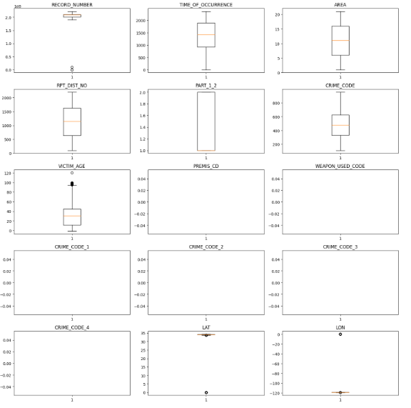
===Boxplot===
They are particularly useful for understanding the range and interquartile range of the data, as well as identifying outliers and comparing data between groups.
In the following, we want to plot multiple boxplots using the subplots method and the boxplot method:

<syntaxhighlight lang="Python" line>
# Create a figure with a grid of subplots
fig, axs = plt.subplots(5, 3, figsize=(15, 15))
# Iterate over the columns and create a boxplot for each one
for i, col in enumerate(numeric_columns.columns):
ax = axs[i // 3, i % 3]
ax.boxplot(numeric_columns[col])
ax.set_title(col)
# Adjust the layout and show the plot
plt.tight_layout()
plt.show()

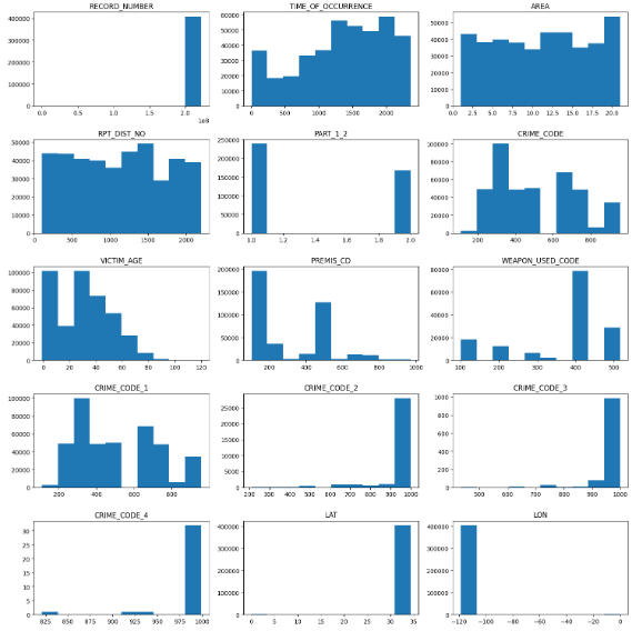
Histogram

Histograms are a type of graphical representation that shows the distribution of a dataset. They are particularly useful for understanding the shape of a distribution and identifying patterns, trends, and anomalies in the data. In the following, we want to plot multiple histograms using the subplots method and the hist method:

12/23/22, 4:25 PM Data_Inspection_ASDA_Wiki - Jupyter Notebook
localhost:8888/notebooks/1000/Data_Inspection_ASDA_Wiki.ipynb 9/9
In [15]:
At this point, we have most of the information needed to start the Data Cleaning process.
# Create a figure with a grid of subplots
fig, axs = plt.subplots(5, 3, figsize=(15, 15))
# Iterate over the columns and create a histogram for each one
for i, col in enumerate(numeric_columns.columns):
ax = axs[i // 3, i % 3]
ax.hist(numeric_columns[col])
ax.set_title(col)
# Adjust the layout and show the plot
plt.tight_layout()
plt.show()

At this point, we have most of the information needed to start the data-cleaning process.

The author of this entry is Sian-Tang Teng. Edited by Milan Maushart